
by Greg Goodman
Inappropriate use of linear regression can produce spurious and significantly low estimations of the true slope of a linear relationship if both variables have significant measurement error or other perturbing factors. This is precisely the case when attempting to regress modelled or observed radiative flux against surface temperatures in order to estimate sensitivity of the climate system.
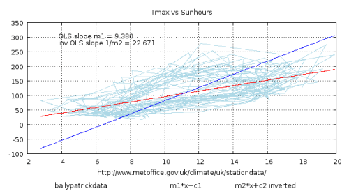
Figure 1 showing conventional and inverse ‘ordinary least squares’ fits to some real, observed climate variables.
Ordinary least squares regression ( OLS ) is a very useful technique, widely used in almost all branches of science. The principal is to adjust one or more fitting parameters to attain the best fit of a model function, according to the criterion of minimising the sum of the squared deviations of the data from the model.
It is usually one of the first techniques that is taught in schools for analysing experimental data. It is also a technique that is misapplied almost as often as it is used correctly.
It can be shown, that under certain conditions, the least squares fit is the best estimation of the true relationship that can be derived from the available data. In statistics this is often called the ‘best, unbiased linear estimator’ of the slope. (Those, who enjoy contrived acronyms, abbreviate this to “BLUE”.)
It is a fundamental assumption of this technique that the ordinate variable ( x-axis ) has negligible error: it is a “controlled variable”. It is the deviations of the dependant variable ( y-azix ) that are minimised. In the case of fitting a straight line to the data, it has been known since at least 1878 that this technique will under-estimate the slope if there is measurement or other errors in the x-variable. (R. J. Adcock) [link]
There are two main conditions for this result to be an accurate estimation of the slope. One is that the deviations of the data from the true relationship are ‘normally’ or gaussian distributed. That is to say that they are of a random nature. This condition can be violated by significant periodic components in the data or excessive number of out-lying data points. The latter may often occur when only a small number of data points is available and the noise, even if random in nature, is not sufficiently sampled to average out.
The other main condition is that there be negligible error ( or non-linear variability ) in the x variable. If this condition is not met, the OLS result derived from the data will almost always under-estimate the slope of the true relationship. This effect is sometimes referred to as regression dilution. The degree by which the slope is under-estimated is determined by the nature of the x and y errors but most strongly by those in x since they are required to be negligible for OLS to give the best estimation.
In this discussion, “errors” can be understood to be both observational inaccuracies and any variability due to some factor other than the supposed linear relationship that it is sought to determine by regression of the two variables.
In certain circumstances regression dilution can be corrected for, but in order to do so, some knowledge of the nature and size of the both x and y errors has to be known. Typically this is not the case beyond knowing whether the x variable is a ‘controlled variable’ with negligible error, although several techniques have been developed to estimate the error in the estimation of the slope [link].
A controlled variable can usually be attained in a controlled experiment, or when studying a time series, provided that the date and time of observations have been recorded and documented in a precise and consistent manner. It is typically not the case when both sets of data are observations of different variables, as is the case when comparing two quantities in climatology.
One way to demonstrate the problem is to invert the x and y axes and repeat the OLS fit. If the result were valid, irrespective of orientation, the first slope would be the reciprocal of second one. However, this is only the case when there is very small errors in both variables, ie. the data is highly correlated ( grouped closely around a straight line ). In the case of one controlled variable and one error prone variable, the inverted result will be incorrect. In the case of two datasets containing observational error, both results will be wrong and the correct result will generally lie somewhere in between.
Another way to check the result is by examining the cross-correlation between the residual and the independent variable ie. ( model – y ) vs x , then repeat for incrementally larger values of the fitted ratio. Depending on the nature of the data, it will often be obvious that the OLS result does not produce the minimum residual between the ordinate and the regressor, ie. it does not optimally account for co-variability of the two quantities.
In the latter situation, the two regression fits can be taken as bounding the likely true value but some knowledge of the relative errors is needed to decide where in that range the best estimation lies. There are a number of techniques such as bisecting the angle, taking the geometric mean (square root of the product), or some other average, but ultimately, they are no more objective unless driven by some knowledge of the relative errors. Clearly bisection would not be correct if one variable had low error, since the true slope would then be close to the OLS fit done with that quantity on the x-axis.
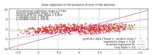
Figure 2. A typical example of linear regression of two noisy variables produced from synthetic randomised data. The true known slope used in generating the data is seen in between the two regression results. ( Click to enlarge graph and access code to reproduce data and graph. )

Figure 2b. A typical example of correct application of linear regression to data with negligible x-errors. The regressed slope is very close to the true value, so close as to be indistinguishable visually. ( Click to enlarge )
The larger the x-errors, the greater the skew in the distribution and the greater the dilution effect.
An Illustration: the Spencer simple model
The following case is used to illustrate the issue with ‘climate-like’ data. However, it should be emphasised that the problem is an objective mathematical one, the principal of which is independent of any particular test data used. Whether the following model is an accurate representation of climate ( it is not claimed to be ) has no bearing on the regression problem.
In a short article on his site Dr. Roy Spencer provided a simple, single-slab ocean, climate model with a predetermined feedback variable built into it. He observed that attempting to derive the climate sensitivity in the usual way consistently under-estimated the know feedback used to generate the data.
By specifying that sensitivity (with a total feedback parameter) in the model, one can see how an analysis of simulated satellite data will yield observations that routinely suggest a more sensitive climate system (lower feedback parameter) than was actually specified in the model run.
And if our climate system generates the illusion that it is sensitive, climate modelers will develop models that are also sensitive, and the more sensitive the climate model, the more global warming it will predict from adding greenhouse gasses to the atmosphere.
This is a very important observation. Regressing noisy radiative flux change against noisy temperature anomalies does consistently produce incorrectly high estimations of climate sensitivity. However, it is not an illusion created by the climate system, it is an illusion created by the incorrect application of OLS regression. When there are errors on both variables, the OLS slope is no longer an accurate estimation of the underlying linear relationship being sought.
Dr Spencer was kind enough to provide an implementation of the simple model in the form of a spread sheet download so that others may experiment and verify the effect.
To demonstrate this problem, the spreadsheet provided was modified to duplicate the dRad vs dTemp graph but with the axes inverted, ie. using exactly the same data for each run but additionally displaying it the other way around. Thus the ‘trend line’ provided by the spreadsheet is calculated with the variables inverted. No changes were made to the model.
Three values for the predetermined feedback variable were used in turn. Two values: 0.9 and 1.9 that Roy Spencer suggests represent the range of IPCC values and 5.0 which he proposes as a value closer to that which he has derived from satellite observational data.
Here is a snap-shot of the spreadsheet showing a table of results from nine runs for each feedback parameter value. Both the conventional and the inverted regression slopes and their geometric mean have been tabulated.
http://climategrog.files.wordpress.com/2014/03/spencer_model.png
Figure 3. Snap-shot of spreadsheet, click to enlarge.
Firstly this confirms Roy Spencer’s observation that the regression of dRad against dTemp consistently and significantly under-estimates the feedback parameter used to create the data in the first place (and hence over-estimates climate sensitivity of the model). In this limited test, error is between a third and a half of the correct value. There is only one value of the conventional least squares slope that is greater than the respective feedback parameter value.
Secondly, it is noted that the geometric mean of the two OLS regressions does provide a reasonably close to the true feedback parameter, for the value derived from satellite observations. Variations are fairly evenly spread either side: the mean is only slightly higher than the true value and the standard deviation is about 9% of the mean.
However, for the two lower feedback values, representing the IPCC range of climate sensitivities, while the usual OLS regression is substantially less than the true value, the geometric mean over-estimates and does not provide a reliable correction over the range of feedbacks.
All the feedbacks represent a net negative feedback ( otherwise the climate system would be fundamentally unstable ). However, the IPCC range of values represents less negative feedbacks, thus a less stable climate. This can be seen reflected in the degree of variability in data plotted in the spreadsheet. The standard deviations of the slopes are also somewhat higher. This can be expected with less feedback controlling variations.
It can be concluded that the ratio of the proportional variability in the two quantities changes as a function of the degree of feedback in the system. The geometric mean of the two slopes does not provide a good estimation of the true feedback for the less stable configurations which have greater variability. This is in agreement with Isobe et al 1990 [link] which considers the merits of several regression methods.
The simple model helps to see how this relates to Rad / Temp scatter plots and climate sensitivity. However, the problem of regression dilution is a totally general mathematical result and can be reproduced from two series having a linear relationship with added random changes, as shown above.
What the papers say
A quick review of several recent papers on the problems of estimating climate sensitivity shows a general lack of appreciation of the regression dilution problem.
Dessler 2010 b [link] :
Estimates of Earth’s climate sensitivity are uncertain, largely because of uncertainty in the long-term cloud feedback.
Spencer & Braswell 2011 [link]:
Abstract: The sensitivity of the climate system to an imposed radiative imbalance remains the largest source of uncertainty in projections of future anthropogenic climate change.
There seems to be agreement that this is the key problem in assessing future climate trends. However, many authors seem unaware of the regression problem and much published work on this issue seems to rely heavily on the false assumption that OLS regression of dRad against dTemp can be used to correctly determine this ratio, and hence various sensitivities and feedbacks.
Trenberth 2010 [link]:
To assess climate sensitivity from Earth radiation observations of limited duration and observed sea surface temperatures (SSTs) requires a closed and therefore global domain, equilibrium between the fields, and robust methods of dealing with noise. Noise arises from natural variability in the atmosphere and observational noise in precessing satellite observations.
Whether or not the results provide meaningful insight depends critically on assumptions, methods and the time scales ….
Indeed so, unfortunately he then goes on to contradict earlier work by Lindzen and Choi that did address the OLS problem including a detailed statistical analysis comparing their results, by relying on inappropriate use of regression. Certainly not an example of the “robust methods” he is calling for.
https://climategrog.files.wordpress.com/2016/03/lc2011_fig7c1.png
Figure 4. Excerpt from Lindzen & Choio 2011, figure 7, showing consistent under-estimation of the slope by OLS regression ( black line ).
Spencer and Braswell 2011 [link]
As shown by SB10, the presence of any time-varying radiative forcing decorrelates the co-variations between radiative flux and temperature. Low correlations lead to regression-diagnosed feedback parameters biased toward zero, which corresponds to a borderline unstable climate system.
This is an important paper highlighting the need to take account of the lagged response of the climate during regression to avoid the decorrelating effect of delays in the response. However, it does not deal with the further attenuation due to regression dilution. It is ultimately still based on regression of two error laden-variables and thus does not recognise regression dilution that is also present in this situation. Thus it is likely that this paper is still over-estimating sensitivity.
Dessler 2011 [link]:
Using a more realistic value of σ(dF_ocean)/σ(dR_cloud) = 20, regression of TOA flux vs. dTs yields a slope that is within 0.4% of lamba.
Then in the conclusion of the paper, emphasis added:
Rather, the evolution of the surface and atmosphere during ENSO variations are dominated by oceanic heat transport. This means in turn that regressions of TOA fluxes vs. δTs can be used to accurately estimate climate sensitivity or the magnitude of climate feedbacks.
Also from a previous paper:
Dessler 2010 b [link]
The impact of a spurious long-term trend in either dRall-sky or dRclear-sky is estimated by adding in a trend of T0.5 W/m 2/ decade into the CERES data. This changes the calculated feedback by T0.18 W/m2/K. Adding these errors in quadrature yields a total uncertainty of 0.74 and 0.77 W/m2/K in the calculations, using the ECMWF and MERRA reanalyses, respectively. Other sources of uncertainty are negligible.
The author was apparently unaware that the inaccuracy of regressing two uncontrolled variables is a major source of uncertainty and error.
Lindzen & Choi 2011 [link]
[Our] new method does moderately well in distinguishing positive from negative feedbacks and in quantifying negative feedbacks. In contrast, we show that simple regression methods used by several existing papers generally exaggerate positive feedbacks and even show positive feedbacks when actual feedbacks are negative.
… but we see clearly that the simple regression always under-estimates negative feedbacks and exaggerates positive feedbacks.
Here the authors have clearly noted that there is a problem with the regression based techniques and go into quite some detail in quantifying the problem, though they do not explicitly identify it as being due to the presence of uncertainty in the x-variable distorting the regression results.
The L&C papers, to their credit, recognise that regression based methods on poorly correlated data seriously under-estimates the slope and utilise techniques to more correctly determine the ratio. They show probability density graphs from Monte Carlo tests to compare the two methods.
It seems the latter authors are exceptional in looking at the sensitivity question without relying on inappropriate use of linear regression. It is certainly part of the reason that their results are considerably lower than almost all other authors on this subject.
Forster & Gregory 2006 [link]
For less than perfectly correlated data, OLS regression of Q-N against δTs will tend to underestimate Y values and therefore overestimate the equilibrium climate sensitivity (see Isobe et al. 1990).
Another important reason for adopting our regression model was to reinforce the main conclusion of the paper: the suggestion of a relatively small equilibrium climate sensitivity. To show the robustness of this conclusion, we deliberately adopted the regression model that gave the highest climate sensitivity (smallest Y value). It has been suggested that a technique based on total least squares regression or bisector least squares regression gives a better fit, when errors in the data are uncharacterized (Isobe et al. 1990). For example, for 1985–96 both of these methods suggest YNET of around 3.5 +/- 2.0 W m2 K-1 ( a 0.7–2.4-K equilibrium surface temperature increase for 2 ϫ CO2 ), and this should be compared to our 1.0–3.6-K range quoted in the conclusions of the paper.
Here, the authors explicitly state the regression problem and its effect on the results of their study on sensitivity. However, when writing in 2005, they apparently feared that it would impede the acceptance of what was already a low value of climate sensitivity if they presented the mathematically more accurate, but lower figures.
It is interesting to note that Roy Spencer, in a non peer reviewed article, found an very similar figure of 3.66 W/m2/K by comparing ERBE data to MSU derived temperatures following Mt Pinatubo.[link]
So Forster and Gregory felt constrained to bury their best estimation of climate sensitivity, and the discussion of the regression problem in an appendix. In view of the ‘gatekeeper’ activities revealed in the Climategate emails, this may have been a wise judgement in 2005.
Now, ten years after the publication of F&G 2006, proper application of the best mathematical techniques available to correct this systematic over-estimation of climate sensitivity is long overdue.
A more recent study Lewis & Curry 2014 [link] used a different method of identifying changes between selected periods and thus is not affected by regression issues. This method also found lower values of climate sensitivity.
Conclusion
Inappropriate use of linear regression can produce spurious and significantly low estimations of the true slope of a linear relationship if both variables have significant measurement error or other perturbing factors.
This is precisely the case when attempting to regress modelled or observed radiative flux against surface temperatures in order to estimate sensitivity of the climate system.
In the sense that this regression is conventionally done in climatology, it will under-estimate the net feedback factor (often denoted as ‘lambda’). Since climate sensitivity is defined as the reciprocal of this term, this results in an over-estimation of climate sensitivity.
This situation may account for the difference between regression-based estimations of climate sensitivity and those produced by other methods. Many techniques to reduce this effect are available in the broader scientific literature, thought there is no single, generally applicable solution to the problem.
Those using linear regression to assess climate sensitivity need to account for this significant source of error when supplying uncertainly values in published estimations of climate sensitivity or take steps to address this issue.
The decorrelation due to simultaneous presence of both the in-phase and orthogonal climate reactions, as noted by Spencer et al, also needs to be accounted for to get the most accurate information from the available data. One possible approach to this is detailed here: https://judithcurry.com/2015/02/06/on-determination-of-tropical-feedbacks/
A mathematical explanation of the origin of regression dilution is provided here:
On the origins of regression dilution.
JC note: As with all guest posts, keep your comments civil and relevant.

Mine eyes glazeth over.
DS. Grok and then mind following comments even if you do not grok the underlying math. This stuff is important. Science stats screw ups are unforgivable, yet common, in ‘climate science’.
And there are many examples. Mann’s centered PCA always producing a hockey stick from ARIMA red noise being Exhibit 1, thanks to Steve McIntyre and Ross McKitrick. And autocorrelated temp series of any sort ALWAYS produce red noise rather than white (random) noise. A statistical issue known in econometrics since I was a ‘grad’ student way back when.
Does this seem like a reasonable venue to you for an article like this?
If so you need to think again. I have neither the time nor skill to vet it. So I’m supposed to trust a few cheerleaders on this blog to do that? Spare me. This should be submitted to a journal not the general public.
Well if you are not capable of following a simple article like that you’re probably wasting you time here.
Your comments are therefore equally worthless. Spare US !
Since this problem has been known for at least 120 years, I don’t think it would get far as a submission to a statistics journal and with the current editor of Nature having declared the debate is over I don’t see much hope of getting correction to anything published by them on the subject.
However, Judith has about 2500 people ‘following’ Climate Etc. most of the them presumably more technically competent than your good self.
Hopefully it will get noticed by some of those who would benefit from being aware of the issue.
Are you a recognized expert in statistics, Greg, or do you just play one on blogs with low standards for guest authors?
Well, I know enough to fit a straight line, so that puts be ahead of the pack , apparently. Since you admit you can’t even follow that much you you should probably stop wasting space and go walk the dog or something.
Haven’t got the time or the skill? You seem to have plenty of time so I guess its the other quality you are critically short of. Not that anyone would have guessed if you have not told us.
“This should be submitted to a journal not the general public.”
I agree with Greg here. This is a well-known problem since way back. You can’t use OLS if there is uncertainty in the X-variable. I have “always known that”, but then I was trained as a physicist, not a climate scientist.
Threatened self-esteem accounts for a large portion of conflict at the individual level.
Nevertheless, David, when you make compensatory remarks like “blogs with low standards for guest authors” and “it’s a pretty f*cking low opinion bolstered by your inability to publish any of this pap on anything more substantial than personal blogs,” do you really believe that’s a good strategy to win hearts and minds?
Some of us like the party here just fine, and are not anxious to see it busted up.
“Kids party goes badly wrong after vicious catfight between mums”
True, true, as a religious leader Mann perhaps had a great deal of influence over his sycophantic followers. But as a scientist you are not supposed to teach how to produce a flood of hockey stick-shaped graphs by simply feeding white noise into a mathematical model that works like a maniacal global warming doomsday machine stuck in maximum overdrive.
Actually, as someone who usually refers to sadistics rather than statistics, I found this post very well explained. I am not sure why the slope would always be under-estimated if the x- axis is not linear, but the fact that an OLS cannot give a correct measure in such a case is – almost – obvious.
Thank you, Greg, for your work. It explains quite a bit of the discrepancy between the different methods of estimating climate sensitivity.
“Actually, as someone who usually refers to sadistics rather than statistics… ”
_____
Thank you, Rob. That made me laugh.
—–
David Springer: This should be submitted to a journal not the general public.
It is too well known for that.
Glen, does it seem to you that I’m concerned with winning hearts and minds here? If so I’d sure like to know what makes you believe that. I could write articles for this blog if I wanted to. Curry would okay them she isn’t picky or critical of what appears under her logo. But I won’t because I’m not an expert in any of the fields relevant to climate science and I’d be ashamed of myself for posing as one. So I confine myself to commentary. I don’t respect others who take advantage of Curry’s lack of discrimination by posing as experts where they clearly are not. In general that legitimizes the complaints from the usual suspects that few recognized experts in the field disagree with the manufactured consensus position.
I’m not an expert in statistics. Neither is Goodman. Foster Grant is a recognized expert in statistics and I read his opinion of Goodman. I evidently know enough about statistics to have arrived at the same opinion as Grant with regard to the competence of Goodman. The giveaway for me was the asinine opinion of Goodman’s that land surface temperature records taken in the air five feet above ground can’t be averaged with sea surface temperature taken five feet below the water’s surface with any meaningful result. That reflects a deep ignorance of the ocean and maritime boundary layer. If he’s willing to put his ignorance on display there he’s willing to do it anywhere. Anywhere including statistics.
While I’m no expert in physical oceanography I did take Introduction to Physical Oceanography in college and got a perfect score in the class with little effort. I spent a long weekend reading the entire physical oceanography textbook and then just showed up in class for midterm and final reviews and exams. And yes, it is just that easy for me. Always has been. That’s as much as I needed to know to arrive at an accurate opinion of Goodman that was subsequently confirmed by a recognized expert in the art of statistics who had occasion to give an opinion on Goodman.
I learned this in a year-long statistics course way back when.
Sounds like some scientists didn’t follow your path. This is not the first criticism I’ve read about the proper use of math/statistics in the field. Other professions have boards to pass minimum proficiency standards.
Maybe we could have a Common Core initiative for climatologists. A natural for some party’s platform.
Well crescokid – I think you just outdid me for comment of the day. Common core for climatologists may just be the answer! Hoisted on their own petard, so to speak.
In 2007 the American Statistical Association’s statement on climate change endorsed the IPCC’s conclusions. I’m not aware of change in the Association’s stance. Does anyone here know of anything more recent?
Max
Does that necessarily endorse all the hundreds of papers beyond the purview of the IPCC? Regardless of how narrow or broad this problem is, why not try to clean it up. If only to remove any cloud of illegitimacy, it seems warmists should want to use the most defensible methods available.
cerescokid March 10, 2016 at 8:56 am
Max
Does that necessarily endorse all the hundreds of papers beyond the purview of the IPCC.
______
Of course not. But the ASA doesn’t say climate science in general is plagued by bad statistical practices as some climate skeptics seem to believe.
Enough individual statisticians disagree to expose the politically correct falsehood espoused by the organization. The organizations are bureaucracies Maxie. Like any other bureaucratic organization political goals that foster the growth of the bureaucracy trump blunt honesty in public statements. Bureaucracies exist to benefit the bureau first. That’s how they survive. It’s really very Darwinian when you think about it.
“I learned this in a year-long statistics course way back when.”
Sadly most climate scientists seem to have little or no formal training in how to process data. They just pick it up as they go along or make up new techniques themselves that they don’t have the wherewithal to validate before using in publishing results.
Since, by definition, peer review is done by their peers, the review process is blind to the problem too.
Greg,
“Sadly most climate scientists seem to have little or no formal training in how to process data.”
_____________
How do you know?
Its an opinion by Greg. Operative words are “most” and “seem”. We don’t “know” anything unless its “settled science” and even then a pinch of salt should be metaphorically taken!
If poor statistical practice is pervasive in climate science why doesn’t the American Statitical Association call attention to the problem and try to do something about it? The Association recently took the bold step of critisizing the p-value, so why not take issue with the way climate scientists use statistics?
Max
Are their offices in the Vatican? Are they the Pope? What does their charter say. Are they the nanny state for users of statistics.
If an entity is using poor statistics in their operations, I hope the Association doesn’t sit outside waiting to barge in to enlighten the transgressors. Their staff would be overwhelmed to paralysis if their mission was to bring compliance with best practices.
Join the real world.
max10k:
By criticizing misuse of p-values the ASA is simultaneously criticising climate researchers (and publishers) who default to 0.5 as “proof” of significance (both statistical and scientific). Or, in the case of Karl’s “pause buster”, the less stringent 0.10 level.
cerescokid | March 11, 2016 at 7:47 am |
Max
Are their offices in the Vatican? Are they the Pope? What does their charter say. Are they the nanny state for users of statistics.
____________
Does the Cisco Kid not know American Statistical Association has an Advisory Committee on Climate Change Policy?
The ASA Advisory Committee is supposed to “Inform Congress, the public, and others on climate change science.”
“It will seek requests from congressional staff for statisticians’ perspective on aspects of the science of climate change and its impacts.
https://www.amstat.org/committees/commdetails.cfm?txtComm=ABTARS01
For activities of the Committee, go to http://www.amstat.org/committees/ccpac/
opluso | March 11, 2016 at 9:20 am |
“By criticizing misuse of p-values the ASA is simultaneously criticising climate researchers (and publishers) who default to 0.5 as “proof” of significance (both statistical and scientific). Or, in the case of Karl’s “pause buster”, the less stringent 0.10 level.’
__________
Either opluso never read the ASA statement on p-values or read it but didn’t understand what he was reading.
Is opluso also unaware the ASA endorses the IPCC’s conclusions?
Yes, but what does that have to do with p-values?
https://www.amstat.org/newsroom/pressreleases/P-ValueStatement.pdf
It’s not about statistics.
“It’s not about statistics”
Very true- It is about unsupported beliefs. There is no reliable evidence that AGW will result in a climate worse for the USA or the world.
Many BELIEVE a warmer world must be worse based on propaganda. Not at all unlike many religious belief systems.
It’s not about that either.
Wrong. It’s precisely about that.
The “abuse” of p-values has been of particular concern in medical research. That does not mean that climate research gets a pass if it incorrectly presents p-values as confirming a hypothesis, etc.
opoluso, I’m sorry if I did’nt make myself clear. I was referring to following part of the ASA President’s comment in the ASA statement on p-values.
“This apparent editorial bias leads to the ‘file-drawer effect,’ in which research with statistically significant outcomes are much more likely to get published, while other work that might well be just as important scientifically is never seen in print.”
http://www.eurekalert.org/pub_releases/2016-03/asa-asa030116.php
My question is do statistical hurdles in general prevent important scientific work from being published?
Wrong. It’s precisely about that.
Yeah, precisely. LMAO.
max10k “My question is do statistical hurdles in general prevent important scientific work from being published?”
That is a good question. There are a number of climate science papers that use “novel” statistical methods which should be considered by the statistical field before they are used in another field. In climate science there is a huge blend of specialties used but there doesn’t seem to be peer review by specialty.
I know of one case where a statistician that developed a method criticized a climate scientist that appeared to misapply the method, but nothing happened.
What it is about is multiple lines of evidence. What it is about is non-reliance on a single study, or a small group of authors. Take him/her/them away, same answer. It is a large number of scientists working on a wide array of climate subjects who are developing and widening multiple lines of evidence.
The pause never stood a chance. Nor does skepticism. You are about to be rolled under… by multiple lines of rapidly growing evidence, almost all of which is pointing… upwards.
http://www.worshipunashamed.org/wp-content/uploads/2012/08/praise.jpg
JCH, “What it is about is multiple lines of evidence.”
“If the glove don’t fit, you must acquit.”
Multiple lines of evidence indicate that CO2 doubling will produce about a degree of warming and zippo else. That about one C degree of warming will occur at some surface still being determined. How much “natural” variability there might be and over what time frames it will be realized is also still being determined. How effective any plan to combat the uncertain amount of warming that is in store is also still being determined.
Since climate science is more like a trial than “normal” science, you have to deal with the wonderful methods used by the legal system.
CO2 might be bad – yep
CO2 might be good – yep
Marcott might be right – yep
Marcott is wrong – yep
result – no action at least no heroic action. Deal with low hang fruit.
btw, http://redneckphysics.blogspot.com/2016/03/uncertainty-in-uncertainty.html
Could this be perjury or just unreliable testimony?
About to be rolled under… an example.
JCH, “About to be rolled under… an example.”
You mean like a kangaroo court? Best evidence right now is about 1.6 C and that assume the past was rock solid stable. Mosher says the past don’t matter, but the past is present as evidence in a post normal science trial. Higher end sensitivities seem to require “novel” methods and each “novel” method should have its own post normal science trial. Its a very ineffective way to do things, but that was the path chosen.
If you want normal science you use normal science. If you want a mockery of a scientific trial, use post normal science and “it;s just so complex!!”
It means:
No single mistake, or small set of mistakes, could notably change the results
The results do not depend on any single fact, data set, model, analysis, investigator, or laboratory
Double dippin dope…
https://www.youtube.com/watch?v=wtLfh3NqNDU
It’s Hip Hop dude
Jch, “It means:
No single mistake, or small set of mistakes, could notably change the results”
That is an assumption not a fact. With Marcott el al. there were quite a few higher resolution reconstructions available to test the validity of his novel method. I just showed one but have looked at about 15 more and they all show the same thing. That paper should not be promoted.
“The results do not depend on any single fact, data set, model, analysis, investigator, or laboratory.”
Basic CO2 physics meets that but the “enhancements” do not. Since Karl et al. modified SST, the 1940s super El Nino is more pronounced and the models have much larger misses during the historical period. That isn’t a single fact etc., that is beginning of a cascade of errors.
In order to validate your position you have to be your own worst critic and not let everything inconvenient slide. In post normal science that would be like concealing evidence which I believe is not Kosher.
a robust test for OLS trends in temperature
http://papers.ssrn.com/sol3/papers.cfm?abstract_id=2631298
Jamal .
“They provide only three values per day – the maximum temperature measured (TMAX), the
minimum temperature measured (TMIN) and an average value for all measurements made during each
day. The actual measurements from which the average was computed are not made available. From
these stations we use only the TMAX and the TMIN values because these values represent actual source”
Tave is (TMAX +tmin) /2
data.
Speak of the devil (people posing as experts) and he appears.
ROFL – still can’t get over you calling yourself a scientist on LinkedIn and me getting a notice from same asking if I knew you. Boy do I.
Jamal .
“They provide only three values per day – the maximum temperature measured (TMAX), the
minimum temperature measured (TMIN) and an average value for all measurements made during each
day. The actual measurements from which the average was computed are not made available. From
these stations we use only the TMAX and the TMIN values because these values represent actual source”
Tave is (TMAX +tmin) /2
data.
GG, a magnificent post. And you touch on only some of the OLS BLUE theorem problems I was taught back when. Heteroscedasticity, sometimes correctable by log normalization. Autocorrelation, sometimes correctible in error terms by ARIMA. Skewness or Kurtosis in error terms, a ‘certain’ diagnostic of BLUE theorem violations, hence OLS unreliability (since BLUE errors should be normally distributed).
IMO, the availability of simple stat packs doing all the calcs mindlessly now, vitiates all the painful ‘what could go wrong’ deep knowledge stuff back when we were crudely programming OLS stuff ourselves. And that lack of deep stats knowledge is the sharp point of your very pointed post.
Regards.
thanks Ristivan, you are correct about stats packages. All people do it look up function, what arguments to feed it, and bang! No one bothers to find out when an where a method is applicable. That are not even aware that they should be doing this.
The prime one is spreadsheets like Excel. You click on a menu option “fit trend” and there is no warming that it may not be a valid result. ( About the only thing M$ does not ask you “are you sure” about).
I strongly agree. I originally learnt the basics of statistics as part of a two year mathematics course at university. It was largely theory and not much applications (this was back in the pre-PC era).
Later I took a company-funded course in applied statistics (mostly as related to reliabilty estimates) and I was very surprised at the way that problems and pitfalls were glossed over or simply ignored, and how software packages were used virtually without any understanding of the theory underpinning the methods used.
Get a room, girls.
reptilian envy
David Springer: Get a room, girls.
What is wrong with you today? Greg Goodman gave a compact presentation of a well-known problem in OLS, and supplied relevant climate-related examples. It’s well suited to a range of people interested in climate statistics.
“Get a room, girls.” Your comments are like spittle on the chin of a drunk. I took statistics in college and haven’t used them in years so it’s tough to follow along with this but there is vital information in there for those of us trying to get a handle on some of the technical aspects. I know my understanding isn’t going to reach that of a physicist who uses statistics everyday in his work but it’s still highly valuable information that rounds out a knowledge field that is full of holes.
I am very grateful for the post. Very!
Fercrisakes Daniel this is a poor venue for it. The following looks lovely. Free open source state of the art software, well illustrated.
http://www.comfsm.fm/~dleeling/statistics/text5.html
Microsoft Excel and OpenOffice Calc are more or less interchangeable so the textbook above will work with that too. I prefer Excel myself it’s a lot faster but I’ve used both.
You’re welcome.
Dummie Donnie still has reptiles on the brain. Small minds, small thoughts.
I saw the article and before reading, I searched the page for “heteroscedasticity”. In the 70’s we were taught to scour the SAS and SPSS plots for evidence of this “disqualifier”. But if you didn’t go to class…
Nice job
+1
Thanks much for such a comprehensive post, including a history lesson and links to literature as well as examples. Sharing now ~:-)
So Forster and Gregory felt constrained to bury their best estimation of climate sensitivity, and the discussion of the regression problem in an appendix. In view of the ‘gatekeeper’ activities revealed in the Climategate emails, this may have been a wise judgement in 2005.
More junk speculation.
What are you trying to say is “junk”. ? The gatekeeping and corruption of peer process was clearly exposed in the CRU emails. F&G clearly state their motivation for not clearly exposing a more rigorous result. Were they guilty of junk speculation too?
The only thing that is speculative is whether this self-censorship was “wise” at the time. The speculative nature of that comment is reflected in the wording “this may have been a wise judgement in 2005.”
So you have nothing to say about the mathematical FACT that most of the literature attempting to estimate clmate sensitivity is biased by misapplication of simple, basic stats?
That shows how little your opinion is worth.
The junk JCH was referring to is you speculating about the motivations of Forster and Gregory. You knew what they felt, eh? So you’re a mind reader. Glad to know you have a marketable skill. Problem is the market is a circus sideshow not here.
Perhaps if you ( both ) developed the remarkable skill of READING and bother to READ the F&G paper that I provided a link to, you would be able to make more intelligent and pertinent remarks rather than uniformed, post from the hip, snide.
Just an idea.
Is the following paragraph necessary?
“So Forster and Gregory felt constrained to bury their best estimation of climate sensitivity, and the discussion of the regression problem in an appendix. In view of the ‘gatekeeper’ activities revealed in the Climategate emails, this may have been a wise judgement in 2005.”
I ask because it isn’t clear whether Forster and Gregory said they “felt constrained to bury ” or this is the author’s opinion. If this is just the author’s opinion, it may raise question’s about his motivation.
Thanks for the civil question Max. Necessary for what?
I could have just posted one line : OLS, please read instructions before opening the packet.
I think that comment is relevant in reviewing the literature on use of OLS in estimating climate sensitivity since the only ones explicitly addressing the issue actually state that they felt doing anything other than repeating the typical error may impede acceptance of their results, which even with this error were on the low end of the market at that time.
This is a rather sad reflection on the state of climatology reflected by insiders publishing in PR journals. They were quite explicitly self- censoring. I think that is relevant
My motivation in writing this? Get those doing OLS to apply it properly and once they get that far, not to self-censor but to publish the best results they are able to produce.
Sorry, but I’m biased.
The following paragraph seems to make my point quite clearly and objectively.
I don’t see any reason to question my motivations … unless those asking the question are seeking distract from the point of the article by going into ad homs.
Spare me the literature bluff, Greggy.
I’ll make it easy for both of us to end this.
Let it suffice as proof of my point upon you failing to quote me the bits from the article where Forster and Gregory talk about the feelings you believe motivated them.
I’m not going hunting for evidence of your claim. Who do you think you are, Steven Mosher? That’s your task. Presumably you are accustomed to failing so I’m sure losing the point will be like water off a duck’s back to you.
Greg
‘Here, the authors explicitly state the regression problem and its effect on the results of their study on sensitivity. However, when writing in 2005, they apparently feared that it would impede the acceptance of what was already a low value of climate sensitivity if they presented the mathematically more accurate, but lower figures.”
“So Forster and Gregory felt constrained to bury their best estimation of climate sensitivity, and the discussion of the regression problem in an appendix. In view of the ‘gatekeeper’ activities revealed in the Climategate emails, this may have been a wise judgement in 2005
The problem is you have no evidence why this was “hidden” in an appendix.
Your supposition:
1. They FEARED it would impede acceptance, therefore they “buried” it in the appendix
The problem is you have no evidence of this fear. The second problem is that it is isnt buried. its right fricken there.
Why does stuff get put on an appendix?
1. You hit the word limit
2. you put it in the main text and a reviewer suggests putting it in the appendix.
3. The reviewer asked you to address the problem and you stuff it in the appendix.
Bottom line, you dont write papers putting stuff in an appendix. It’s the result ( typically) of a negotiation with other authorities.
read the appendix.
“It has been suggested that a technique based on total
least squares regression or bisector least squares regression
gives a better fit, when errors in the data are uncharacterized”
Looking at the appendix and the reference to other uses of bisector
I would bet one of the reviewers was a guy at CRU.
IT HAS BEEN SUGGESTED…. that should be a clue.
Bottomline; When a document has reviewers and editors ANY attribution of motive to the author is limited. We see this all the time in Literature where we have the author’s original text and then the text after editing. In this case you dont have the original text. You dont have the reviewers comments and and editor replies. So, you can’t even begin to argue for authorial intentions.
It’s in the appendix. Crap we put some of our most important stuff in the appendix. In a science text an appendix is NOT a vestigal organ.
.
I posed the question of using total least squares to whoever was the communicating author of Forster and Gregory- I do not recall which one it was – and showed him my results. His reply was that he did not think it was game changer or something to that effect.
As to what is included in the main paper and the SI can be very telling about the authors motivations and whether the author might be willing to bury a weakness in their thesis. If something is in the SI that could be a game changer means that the authors were aware of it but decided to put it in the SI. If a knowledgable reader sees it that way it should raise some antenna. Similar problems are where an obvious sensitivity test was not run and the question that would have presented was entirely ignored.
These situations have been documented in climate science papers and would appear to be more prevalent with authors who tend to be policy advocates.
“As to what is included in the main paper and the SI can be very telling about the authors motivations and whether the author might be willing to bury a weakness in their thesis.”
If the editors demanded that the material be moved to a SI, then what?
You simply cannot divine authorial intention from the structure of a document that is not entirely under there control.
Next people will say that stuff is “hidden” in the code.
The paper is the whole paper and its data.
Now, I could just as well argue that pushing a reading about authorial intention was more TELLING about the reader than the author.
It was Andrews who I corresponded about using TLS regression. What I found using TLS was that the ECS values where considerably larger than those reported by Gregory/Andrews and those I determined using LS regression. My reference to Andrew’s reply is in the second link below and he says that they did not look at using TLS even after it was reported that it might be an issue.
The secondary link in the first link below is to a table with my results using TLS and LS (and not RLS as the table label shows).
http://rankexploits.com/musings/2014/new-open-thread/#comment-134160
http://rankexploits.com/musings/2014/new-open-thread/#comment-134467
“If the editors demanded that the material be moved to a SI, then what?”
The authors should then point to the fact that it would change the importance of the point being made by the comment or result and that it should be left in main paper. If the editors continued to insist it be in the SI then I would have to question their judgment and motives. If it were space limitations then find something else to put in the SI.
It is not that difficult for a person knowledgeable in the area of a paper’s contents to see when something that should be in the main paper is put into the SI. I suppose an ever trusting soul could and probably would always say that it was an editor’s choice. That is another reason that the SI could be a dumping ground for critical comments and results – the author can blame it on the editor or least for the trusting souls..
“If the editors demanded that the material be moved to a SI, then what?”
Simple – you put there and also include a sensitivity analysis. Editor is happy. Mosher and friends can say “It’s all there” and no-one can brush off anyone who asks with a “it’s not significant to the results” because it’s plainly in the SI that it is or isn’t.
If you didn’t do the sensitivity analysis, you can’t use the “it’s not significant” argument – unless you’re God, I suppose. If you HAVE done it, put it in the SI. If you haven’t done it, don’t LIE about what’s important and what’s not – just say, “I/we didn’t test for that”.
Clearly, in this case a sensitivity analysis is NOT in the SI, so at this point, the worst argument against the author is “wasn’t thorough enough” and any arguments about intent, feelings etc are the domain of the spin doctors.
Hear that Mosher? You’re being a SPIN DOCTOR! Yep, picking on something you know you can’t lose on, that is totally irrelevant to the actual SCIENCE. Pay attention to what matters – that’s data and analysis. If you believe that the mention of the authors feelings are undeterminable or whatever, ignore it! Look at the maths. Look at the logic. Consider the implications of THOSE. Admit the man has a point. Do something constructive, same as the main post author attempted to do before you derailed the conversation with dross.
What concerns me is this: when someone else DOES do a sensitivity analysis, past experience says that they get told they are making their own predictions/projections instead – a la Steve Mc. While the consensus says it doesn’t change the conclusions of the paper – which is trivially true, because those conclusions were reached without said analysis. That sort of twisting and word-play to ensure no-one deviates from “the message” is a disgusting attitude for anyone claiming to be a scientist, IMO.
I thought I was good at supposing but I’m out of my league here.
Kneel..
Let’s be clear. I am skeptical that you can prove authorial intentions in this case.
But you seem to think that the science of reading texts is settled.
Go ahead… Prove that they felt fear as Greg claimed.
I can’t figure out the last paragraph is saying:
http://www.theamericanmag.com/uploaded_images/article_1976_2GjxeJdvX3.jpg
“Look at the logic. Consider the implications of THOSE. Admit the man has a point. ”
OF COURSE he has a point.
“Do something constructive, same as the main post author attempted to do before you derailed the conversation with dross.”
Look. in this article and in others Greg has made fine points. He is correct. That is WHY I have a problem with HIM dragging in the
shaky science of divining authorial intentions. If I had to give him
one piece of advice it would be drop the mind reading. People in the comments will “connect the dots”.
I would rather people focus on his statistical issue, but when he has this glaring lapse of judgement about divining intentions, of course people are going to jump on it.
Finally, the sensitivity debate has really moved past the texts he talks about
Ignorant or disingenuous? It’s always the same question, the same question.
==============
Mosher is correct.
If this was a courtroom and Greggy started talking about how someone felt about something the other attorney would quickly say “Objection your honor. Speculation” and the reply from the bench “Sustained”.
Gimpy Greggy the mighty guest blog warrior of course can’t admit his mistake which is typical of his ilk.
PS Mosher that’s vestigial not vestigal. I can’t escape built in spell checkers these days in text editors. Evidently you found a way.
Even my latest adventure into Android Studio the editor is crazy proactive. It annoys the crap out of me spell checking even invented names assigned to methods and variables. I can’t stand having any compiler warnings so it’s doubly annoying changing names just to make it happy. I like my work to build clean using default settings probably to the point where I’d be diagnosed OCD about it otherwise I’d tweak some settings to make it stop.
Nothin’ from nothin’ leaves nothin’
You gotta have somethin’ if you wanna be… [believed!]
Reblogged this on TheFlippinTruth.
Yeahh, and inappropriate use can lead to high estimations as well. Statistics are a blunt tool suited to real correlations in correct relationships. Anything unknown produces equivocal scatter.
Statistics can be useful pointing direction, but ultimately we need to figure out what is going on. When you actually figure out what is going on, statistics fall right into place, just like they were always there.
It is possible to construct a dataset where OLS will over estimate the slope but it’s pretty contrived. The term regression dilution is used because it will almost always reduce the fitted slope. In the case of CS , which is the reciprocal of the rad vs temp slope , this lead to over-estimation of CS.
Yes, I understand this is a legitimate technical criticism akin to “running mean smoothers” a while back. Have done triple running means ever since that one, but since I have little regard for regressions through noisy data…
Figure out what’s going on. The appropriate data will make your regression easy.You’ll never need to worry about dilution.
Right. Relatively greater values of negative feedback suggest lower values of sensitivity and greater stability (as this post shows). But if the feedback is not instantaneous but delayed – as it is with changes in atmospheric and ocean circulation, albedo, etc. – there will be the increasing likelihood of oscillations and ringing; that is, changes to climate not related to forcings but merely the character of a nonlinear, non-equilibrium system – like our planet’s. Kapish?
comments related to the content of the article will be welcome – Mr. Kapish.
Acknowledged. I apologize. I just got so excited…
Herewith kinda’ deja-vu all over again apropos cli-sci-
tricky-methodology … Ross McKitrick, ‘What is the
Hockey Stick Debate About?’ You know, suss proxy
data, cherry picked ‘n weighted samples …Sheep
Mountain anyone? And if that ain’t enuff, that Mann
algorithm that data-mines for hockey sticks.
http://climateaudit.org/2005/04/08/mckitrick-what-the-hockey-stick-debate-is-about/
Another opinion of Greg Goodman. About the same as mine.
https://tamino.wordpress.com/2013/03/08/back-to-school/
Yes, Grant Foster tried to be a bit too smart ( for a change ) and got himself into a situation he could not bluff his way out of. He decided to “win” the argument by banning me from his site and deleting my inconvenient comments. Very ‘open minded’ and scientific.
https://climategrog.wordpress.com/2013/03/11/open-mind-or-cowardly-bigot/
BTW , could you remind us what your opinion of my work is? Just speaking as someone that admits he does not have the skill to understand it, that could be very useful to others.
Oh my. Grant Foster is a recognized expert in data analysis. Astrophysics even.
https://scholar.google.com/scholar?hl=en&q=grant+foster&btnG=&as_sdt=1%2C44&as_sdtp=
Sole author in data analysis relevant work in the Astronomical Journal and Environmental Research Letters. Hundreds and hundreds of citations to his work.
Remind me again, what are your credentials in this field Greggy and where has your work been published?
Given I’m not an expert in statistics I’m going to have trust someone else instead. You or Grant Foster at this point is not a difficult decision.
Did it cross your mind for even a brief instant, Greg, that Grant Foster just didn’t want to waste his time dealing with a nobody holding delusions of competence? It certainly crossed my mind.
I don’t link it because I’m not trying to pull in traffic. It’s not a blog, it’s a work area. Somewhere to stick scripts and graphs I want to refer to. The only things I put there as posts are final drafts for articles like this one that get accepted to other sites that ARE running a blog.
If wanted to waste my days dealing with idiots like you and Tammy I would turn comments on.
Turning comments on until someone disagrees with you is not having comments ‘open’. Calling someone a 1iar and then running to hide behind a locked door is not very impressive behaviour. It is certainly not a sign of having an ‘open mind’ or trying to advance scientific knowledge.
Fine, go ask Grant about how to fit a straight line to a scatter plot and see what he recommends. I’m not forcing you to accept what I say. If you prefer his site go and hang out over there and give everyone on C. Etc a break.
Further… The Astronomical Journal where Foster was sole author in a number of data analysis articles “is one of the premier journals for astronomy in the world”. And of course “Environmental Research Letters” is top shelf as well.
Feel free to point to your accomplishments in this field, Greg, that I may compare them for expertise in statistical data analysis. May the real expert win. Good luck.
No that won’t work. Foster would ban me as quick as you. The difference between you and me is that I won’t fool myself into thinking he banned me because I know more about statistics than he does.
Besides, it’s way more fun here and you’re a sitting duck. Like shooting fish in a barrel.
When I want to be sure that somebody can’t get away with deleting an inconvenient comment stream, I use the Wayback Machine (or other archiving utility as appropriate) to save off a copy for future reference.
(There’s a way they can prevent people from seeing the captured web page, but it also makes that page inaccessible to search engines. Mostly blog owners don’t want that.)
David Springer,
I’m dissapointed. Current climate scientists are “recognized experts” in climate science, but you certainly cannot trust them. They suffer badly from paradigm paralysis and ignore anything but their CO2 knob.
Open Mind is laughable.
David Springer: Given I’m not an expert in statistics I’m going to have trust someone else instead. You or Grant Foster at this point is not a difficult decision.
Greg Goodman is correct on this technical point. consult the appendix Foster and Gregory: For less than perfectly correlated data, OLS regression of Q-N against δTs will tend to underestimate Y values and therefore overestimate the equilibrium climate sensitivity (see Isobe et al. 1990). .
Why prominent users of statistical packages ignore these fundamental problems is a mystery. I posit a Gresham’s law of statistics: Cheap statistics drive thorough statistics out of the market. Think how frequently MBH98 is cited in approbation, without citation of the published correction, which had been stimulated by the critique written by .McIntyre and McKittrick.
matthewrmarler says
I posit a Gresham’s law of statistics: Cheap statistics drive thorough statistics out of the market.
_____________
Some more posits:
Statistics pedants throw out the baby and keep the bath water.
Don’t let the statistics tail wag the science dog.
max10k: Don’t let the statistics tail wag the science dog.
That makes no sense. All phenomena display random variation (variation that is non-reproducible and non-predictable; the distribution can sometimes be known with reasonable accuracy), and statistics is the study of how the random variation affects measurements, estimates, calculations, conclusions, and all inferences generally. Greg Goodman presented a short tutorial on one of the neglected consequences of random variation in the context of linear regression. You can’t increase the precision of knowledge by ignoring the random variability, all you can do that way is increase your error rates.
Back to the earlier question: Is there a reason that tamino is downplaying this problem, given that he and Gregory included it in an appendix to a published paper? I have seen papers where derivations and other details are presented in appendices or supporting online material (e.g. Romps et al), but I have not seen a paper where an important result derived in an appendix was not given prominence in the main text.
matthewrmarler | March 11, 2016 at 12:12 am |
max10k: Don’t let the statistics tail wag the science dog.
That makes no sense
_________
Makes sense to me. Just means don’t get so wrapped up in statistics that you forget statistics is a tool for science, not the objective of science. Read my post here on the recent statement by the ASA.
Back to the earlier question: Is there a reason that tamino is downplaying this problem, given that he and Gregory included it in an appendix to a published paper? I have seen papers where derivations and other details are presented in appendices or supporting online material (e.g. Romps et al), but I have not seen a paper where an important result derived in an appendix was not given prominence in the main text.
Forster of Forster and Gregory is not Tamino.
max10k: Read my post here on the recent statement by the ASA.
I have the document from the ASA and the comments by distinguished statisticians as well (Jim Berger, Rod Little, Greenland et al., Gelman) . I even forwarded them to some colleagues who are not ASA members. Your comments are not that good.
Greg Goosman’s essay did not display misuse of p-values.
In this instance: Greg Goodman showed in his essay that neglecting the uncertainty in the predictors produced a parameter estimate that was in error by enough to materially affect the estimate of an important climate-change-related quantity. That is not the tail wagging the dog. That is an important scientific issue. It is also a well-known problem, and he showed examples of the neglect/disrespect of important statistical problems by climate scientists.
JCH; Forster of Forster and Gregory is not Tamino.
Yes. I was confusing Foster and Forster. rats. bummer. argh. and so on.
A good example of the statistics tail wagging the science dog is p-hacking.
I didn’t say Greg is wagging the dog here. I don’t know. He’s not wagging the dog if what he is saying is a game changer. But he may be if what he’s saying makes little difference.
max10k: I didn’t say Greg is wagging the dog here. I don’t know.
Have you written anything relevant to Greg Goodman’s essay?
Read my first post. I asked Greg a question. He must have thought the question was relevant because he thanked me an replied.
My other posts were in response to comments.
Greg Goodman | March 10, 2016 at 4:09 am |
“If wanted to waste my days dealing with idiots like you and Tammy I would turn comments on.”
Yet here you are doing exactly that.
Greg Goodman | March 10, 2016 at 4:09 am |
“If wanted to waste my days dealing with ***idi0ts like you and Tammy I would turn comments on.”
Yet here you are doing exactly that.
https://www.youtube.com/watch?v=ZBAijg5Betw
The word idi0t, spelled properly with an oh instead of zero triggers moderation. Curry therefore explicitely approved of Greggy’s comment calling denizens idi0ts. I guess that makes it okay for the rest of us.
How odd – a defender of the faith complains, not with references to obvious errors of maths or logic in the post, but instead an attack on the tone and attitude of the post and the “my expert is smarter than yours” retort of a child.
Never saw that before… oh wait…
Based upon your assertion in another article here that land and sea surface temperature records can’t be averaged together into anything meaningful it’s a pretty f*cking low opinion bolstered by your inability to publish any of this pap on anything more substantial than personal blogs. Point to something more substantial and I’ll apologize. Good luck.
You already ARE an appology, Don’t worry about it. In view of you skill set I don’t think it would matter very much if you thought this article was great.
Thanks for sharing !!
Yeah that’s what I thought. All hat, no cattle.
I’ll agree with at least part of you what you wrote above: “I don’t think”. Truer words were never spoken.
Springmiester, “Based upon your assertion in another article here that land and sea surface temperature records can’t be averaged together into anything meaningful it’s a pretty f*cking low….”
Greg could work on his delivery, but combined land and sea average temperature has lots of limitations. You for example tend to harp on “latent” cooling. A large part of that “latent” cooling produces land warming and land warming tends to have an amplification factor different than the surfaces that produced the “latent cooling”. So Jimmy D can “highlight” land warming that is more accurately a mix of radiant cooling (Arctic Winter Warming) and “real” warming approximated by a kludge to fit the not so great data while you wander down the latent cooling hole. With a reliable “index” you and JimmyD would be on the same page.
btw, Mosher has done something up on the RSS 4.0 versus surface temperatures. Oceans are very close, land has the largest difference especially land area that tends to have temperature inversions. RSS agrees more with Tmin than Tmax and there was that weird shift in DTR circa 1985 so Tmax and Tmin trends aren’t following the game plan.
https://andthentheresphysics.wordpress.com/2016/03/08/guest-post-surface-and-satellite-discrepancy/
You’re babbling again, Dallas, just to hear yourself talk. Stop it. Temperature is the single most used practical measure of surface environment. Imagine not knowing it. What would substitute?
So fat my crayons on WfT have not been updated with FEB 2016, so this will have to do (you have to look way up to see Feb) :
https://tamino.files.wordpress.com/2016/03/nasa21.jpeg
Spinger meister, ” What would substitute?”
Energy relevant temperatures. No real problem with SST because the range from ~30 C – ~-2 C is small enough to be relevant. With air temperatures at the “surface” you have a range of ~50 C to -80 C which is much too large a span for a meaningful average and most of the close to -80 C is guess work. Since you are converting to anomaly you would need to weight temperature to effective energy for the anomaly to be meaningful.
Think of it like a heat engine, you use T source and T sink to estimate efficiency not Tave. The ocean average SST is close to T source to be useful, still not great since there is latent etc. but it is a better reference than guesses at Tmin + Tmax over 5% of the globe with next to zero reliable measurements.
Mosher is all like, “We have to fabricate polar temperatures!!” Nope, an index is a reference and should be consistent. If you don’t have data, you don;t have it, deal with it.
JCH, Put down the crayons
http://climexp.knmi.nl/data/igiss_temp_1200_0-360E_-90-90N_n_1910:1940_a.png
Looks like close to the same huge spike that preceded quite a few years of lower than normal temperatures. So either we are done, might as well party or we are in for a few decades of not much to see.
The spike around 1940 was at the end of the ramp up of the PDO. In this case, the PDO may just be firing up. Regardless, I have to have my crayons ready to go at every moment as it’s a complex and chaotic and dynamic system that can surprise at any turn. Don’t blink, you might miss a tipping point, or a regime shift, or… some fish.
JCH, “The spike around 1940 was at the end of the ramp up of the PDO. In this case, the PDO may just be firing up.”
Perhaps, but the rainfall data in California indicates that spike was more likely El Nino related. Hard to separate the two I imagine, but considering how much effort was made to adjust it away, it is kinda neat to see it is back in full form :)
So much anger.
Andrew
David Springer, I’ve noticed you very frequently appeal to the argument from authority. This is a very well established logical fallacy regardless of your expertise or self admittedly lack thereof. Google that up if you are not familiar with that notion.
It would be much more useful to the rest of us if you allowed the other experts to challenge Greg and others with facts and specific points rather than the approach you have taken, which offers no value other than to make it harder to follow those afore mentioned discussions.
I am sure we would all welcome your comments in areas you do bring more expertise.
Regards,
Tad.
No, Tad. Arguments from authority are perfectly legitimate when a real authority in the topic at hand is utilized.
I suppose I should tell you now I took formal logic in college too and got a perfect grade on every single test with very little effort. Most of the class failed. Community college though so the failure rate is somewhat understandable. Those were not typically people who ended up getting paid in the millions like a pro ball-player for their talent at stringing billions of logic gates together into what became the dawn of the information age.
You’re welcome. Here’s your lesson in logic for today (my emphasis so):
https://en.wikipedia.org/wiki/Argument_from_authority
Trust me. I don’t make fallacious appeals to authority. I was very careful to provide the bona fides of my source in the field of both statistics and temperature regression analysis. Grant Foster is a recognized expert with on topic publications in high impact journals, sole author on some with hundreds of citations, to which I linked with google scholar.
https://scholar.google.com/scholar?hl=en&q=%22grant+foster%22&btnG=&as_sdt=1%2C44&as_sdtp=
That my friend is how an appeal to authority is made. Now you know. Or at least you’ve been told.
There seem to be a good number of commenters here who use WoodforTrees without fully appreciating the limitations that Greg has pointed out in the above post. This post, BTW, is an excellent article that I would recommend that everyone should read and I appreciated it. As Judith usually says with guest posts, lets be civil and relevant.
Plus lots ‘n lots Peter.
The x-error problem does not arise in time series themselves since time is usually low error. . However, the presence of significant non linear , pseudo periodic variability is well known and why it always comes down to a cherry-pick as to what result you will get.
https://climategrog.files.wordpress.com/2013/04/warming-cosine.png
https://climategrog.wordpress.com/warming-cosine/
That graph illustrates how you can get ‘accelerated warming’ out of a non trending periodic function, similar to the variations in climate.
So keep the the trends with respect to AMO phase:
http://www.woodfortrees.org/plot/hadsst3gl/from:1900/plot/hadsst3gl/from:1911/to:1976/trend/plot/hadsst3gl/from:1945/to:2010/trend
”The x-error problem does not arise in time series themselves since time is usually low error”
It does, if the data is older than c. 1700 AD, because the dating will then usually be indirect and subject to significant errors. This applies even to the best methods, like varve/treering-counts, AMS radiocarbon dates and interpolation between historically dated ash-layers. This is one of the reasons that the argument that current rates of climatic change are unprececdentedly fast is very dubious.
Greg, that’s exactly what Jones and Trenberth did in one of their misleading graphs in IPCC AR4.
While its true that T is not a problematic as the x error and that Rud’s points covering a few other issues with the use of OLS regression trend estimates have not been covered in Greg’s post, I still consider that climate data would not be considered long enough in terms of time elapsed nor precise enough in terms of spacial coverage for statistical inference about future states of global climate to be.valid.
Clearly extrapolating a model tuned to fit 1960 -1998 out to 2100 is absurd, even if the data was of exceptionally good rather than exceptionally bad quality.
nuts
JCH
Doesn’t quite measure up to Bastogne.
You can write anything on this blog. It’s a cesspool. Nothing else could have this much crap in it.
Hey JCH,
How’s that rhetorical strategy of yours worked out for you and the rest of the climatriat with the American public?
http://i.imgur.com/cHrD4hU.png
You will see some push back against the satellite temperature series before I started calling them garbage here at Climate Etc., but now criticizing the satellite series is a cottage industry on blogs, and the critics are drawing some blood. RSS finally got off its butt and fixed their embarrassment.
Same for my former favorite target of abuse: HadCRAPPY3, the gold standard of a bygone era in climate science… now like a hunk of space junk.
So maybe I’m doing better than you think!
Greg Goodman March 10, 2016 at 5:40 am
“Clearly extrapolating a model tuned to fit 1960 -1998 out to 2100 is absurd, even if the data was of exceptionally good rather than exceptionally bad quality.”
_______
I’m not sure I would call an extrapolated OLS line “absurd.” It is what is.
Here is a paper that appears to be discussing some of this stuff.
Are climate model simulations useful for forecasting precipitation trends? Hindcast and synthetic-data experiments
JCH:
Definitely not civil and, as far as I could tell from your link, not relevant, either.
“You can write anything on this blog. It’s a cesspool. Nothing else could have this much crap in it.”
So much anger.
Andrew
JCH
Have you toured your local municipal sewer plant lately?
JCH: Nothing else could have this much crap in it.
Except possibly for the speculation (which may be correct) of why Foster and Gregory put their most important result in the appendix where almost everyone would ignore it, the presentation by Greg Goodman is pretty good.
JCH March 10, 2016 at 12:25 pm
“Here is a paper that appears to be discussing some of this stuff.”
No “Are climate model simulations useful for forecasting precipitation trends? Hindcast and synthetic-data experiments” Nir Y Krakauer and Balázs M Fekete isn’t discussing this stuff.
What it does (concentrating on where it uses observational data) is construct 4 ways of forecasting precipitation trends for periods from 1960 all ending in 2010 (lengths from 1 to 50 years). The 3 non-GMC ways they know nothing about the period being forecast (“Based on available data up to a time t1 and GCM simulations, our objective was to hindcast [sic] the precipitation change P ¯(t2) − P ¯(t1) for various times t2 > t1”). On the other hand the GCM method was done by fitting “a smoothing cubic spline .. using the entire run from 1901 to 2010”.
Somewhat unsurprisingly the GCM method did better.
Regrettably they failed to show as per their conclusion “Our hindcast and forecast experiments suggest that climate models have some skill in simulating precipitation change over the next few decades.” They showed instead that if one uses the information about the period you are purporting to predict, and fit a more sophisticated curve, you get better results than doing it blind with a simple straight line (or fixed value).
Is Environmental Research Letters peer reviewed?
JCH – the most important metric is almost certainly rate of change in ocean heat content. The signal is believed to be on the order of 0.5W/m2 more energy at top of atmosphere entering the system than is exiting which, because the ocean is by far the major solar heat reservoir, is roughly equivalent to how much the ocean is warming. The margin of error in measurment is +-4.0W/m2. Figure it out. We have to guess at the polarity using proxy measurements with similar physical inaccuracies like ocean level and arctic ice extent. Oh it must be warming because look at the ice melting. Right.
Be that as it may it gets worse. We don’t know very well how energy moves around verticially or horizontally in the ocean. The commonly quoted TOA imbalance of 0.5W/m2 is only enough to raise the temperature of the ocean’s entire volume by 0.2C in one hundred years. We know the excess solar energy (if it exists) must be absorbed virtually entirely in the first 100 meters of the ocean where it is converted to kinetic (thermal) energy. How it moves from there becomes a big mystery and therein lies the answer to the $64,000 climate question because it’s the difference between the top 10% of the ocean rising 2C in 100 years on one extreme or it rising 0.2C on the other.
One is potentially bad news and the other not noticeable. Where the ocean surface temperature goes so does the air nearest the surface, including over land to a large degree due to rapid horizontal mixing of energy in the atmosphere in the way of moist air masses from the ocean rolling across the continents releasing vast amounts of energy along the way in latent heat of fusion (condensation).
Maybe it’s just me but I figure it’s pretty important to know whether 100 years of global warming at current best measurement of rise in OHC is going to be noticeable or not.
Peter M Davies March 10, 2016 at 4:36 am
There seem to be a good number of commenters here who use WoodforTrees without fully appreciating the limitations that Greg has pointed out in the above post.
——————————–
All I have seen is commenters using OLS in woodfortrees to express temperature change as a function of time. Aside from cherry picking points in time, I see nothing wrong with that. I believe Greg agrees.
–
OLS regression performed on short time-series will produce a pretty graph of a trend line and even if we leave the issue of cherry picking aside, these lines do not prove anything about where global climate is heading over the next decade or two. When we have a 100 years of reliable satellite data I would, if alive, be prepared to discuss short term trends either way.
Extrapolating an OLS will give you a naive projection or forecast, which may or may not turn out to be more accurate than a no-change extrapolation. I don’t think any forecasts are supposed to “prove” what will happen in the future.
From what I’ve seen, readers here at ClimateEtc use woodfortrees just to study what has happened rather than forecast.
I agree completely with what you have just said Max and with what you say in general more often than not. My problem is the alarmism that is being promulgated from such tenuous data and the policy proposals that are being put forward as mandatory on western economies.
Can you even use WFT to make forecasts, at least insofar as it can plot the graphs?
I don’t think you can use woodfortrees to extrapolate an OLS line, but I haven’t been there lately.
If you want to do blind statistics to suggest stuff, which is okay, MDSCAL is probably a good thing to look into.
It has the advantage of being nonparametric.
Of course, if R**2 is only 0.019, we’re talking about a damned scatter plot anyway (see Figure 3). To me, that’s a much bigger flaw in most of the models – not misusing OLS, but using it at all. The assumption of linearity seems foolish in the extreme when there are so many interdependent phenomena going on.
A recently released statement by the American Statistical Association seems relevant.
‘The American Statistical Association (ASA) has released a “Statement on Statistical Significance and P-Values” with six principles underlying the proper use and interpretation of the p-value. The ASA releases this guidance on p-values to improve the conduct and interpretation of quantitative science and inform the growing emphasis on reproducibility of science research.’
The following are comments by the ASA’s executive director and president.
“The p-value was never intended to be a substitute for scientific reasoning,” said Ron Wasserstein, the ASA’s executive director. “Well-reasoned statistical arguments contain much more than the value of a single number and whether that number exceeds an arbitrary threshold. The ASA statement is intended to steer research into a ‘post p<0.05 era.'"
"Over time it appears the p-value has become a gatekeeper for whether work is publishable, at least in some fields," said Jessica Utts, ASA president. "This apparent editorial bias leads to the 'file-drawer effect,' in which research with statistically significant outcomes are much more likely to get published, while other work that might well be just as important scientifically is never seen in print. It also leads to practices called by such names as 'p-hacking' and 'data dredging' that emphasize the search for small p-values over other statistical and scientific reasoning."
http://www.eurekalert.org/pub_releases/2016-03/asa-asa030116.php
JCH | March 10, 2016 at 9:44 am |
About 75% of the comments on C.,E., seem to be dominated by three names JDC, JimD and David Springer. You can help reduce the amount of “crap” here any time you like.
You and Jim are simply ignorant about science, which is excusable, yet refuse to learn and come back with the same garbage day after day. That is not.
Springer is just a troll, who admits he knows nothing and has too much time on his hands.
That does waste a lot of bandwidth and is wasting huge amounts of “carbon”. Please stop , we must save the Earth , now.
First let me admit that my statistics is very limited but I get the idea of a tightly constrained x-axis (e.g. time of observation) vs. a Y- axis where there is significant error or variability.
If I understand correctly then the use of an ordinary least squares regression would be incorrect in the following example. Say I am calculating the historic rate of sea-level rise in an area using the depth of dead tree stumps below the present high water mark versus time (- y). Here there is error in determining the average high water mark (tide gauges are few and far between) and you might have to use the seaweed strand line (subject to varying tidal range and recent storm waves.
Time is measured by C14 dating of the stump. This is the x-axis. However a typical C14 date has an error of +/- 40 years. In addition, the actual age isn’t age +/- error, rather it has an additional error range in that the actual age is a range or statistical probability range due to variations of C14 vs. fluctuating cosmic rays.
Since there is considerable error in both x and y the use of the OLS method would yield rates of sea-level rise that are to low. ??
Short answer, yes, it is likely. How much depends on the structure and size of the errors in each variable. You could try making some synthetic data using suitably scaled random numbers to make similar data with and with errors in the dates. Then do lots of runs to see how much it typically degrades the slope ( which you know in advance since you programmed it in.
If you click on fig. 2 you will find a script to make some trial data that you may be able to adapt.
It still sounds like your time errors will quite a bit smaller than the y errors so some of the other methods like bisecting the two slopes seen in fig 2 or taking the geometric mean may go too far the other way. It’s actually quite hard to know how to get a better result but at least being aware of the problem avoids have too much faith is a probably distorted result.
Phillip, This might be a pretty good example for you.
https://lh3.googleusercontent.com/-XWxUtSoLgJg/VHOWejsl5JI/AAAAAAAAL0Q/FuQL-0CIV2I8CXnmQNwv6Pu28QRfTgjUQCCo/s577-Ic42/IPWP%2Boppo%2Bwith%2Bm.png
Both reconstructions are from the same place with different sampling times. The Mothadi 2010 has about 400 years between samples and the Oppo 2009 about 50 years between samples. The Mothadi data was used by Marcott et al who tried time jiggling to reduce uncertainty. Doesn’t look like it would work very well.
I am surprised that nobody has yet mentioned one of the most spectacularly inappropriate misuses of regression, Lewandowsky’s bogus attempt to imply that climate sceptics are conspiracy theorists.
It’s nicely illustrated by the picture on page 27 of Brandon’s recent e-book.
Maybe somebody could be bothered to pick out the image and post it.
As most people here probably know, L and co found that most climate change believers don’t think the moon landing was faked, and drew the false conclusion that climate sceptics do, based on only 3 out of 1145 responses.
In addition to being labeled a liar, a criminal and a hacker, my examination of these topics has also gotten me labeled a conspiracy nut.
I”m not the only one. Every person who speaks out at all against the consensus message gets labeled the same way.
It all started with a paper titled:
Whose lead author was a man named Stephan Lewandowsky.
The story behind this paper would take too much time to explain here, but the incredible thing about the paper is only 10 of the 1,145 peole surveyed claimed to believe the moon landing had been faked.
Of those 10, seven endorsed the global warming consensus position.
Only three out of 1,145 people claimed to be skeptical of global warming and believe the moon landing had been faked, yet this paper portrayed all global warming skeptics as conspiracy nuts, claiming to have found a statistically significant correlation between being a global warming skeptic and a conspiracy nut.
So how did they do it? Take a look at this image to see:
http://i.imgur.com/CGyE8Jf.png
The diagonal line represents the supposed relation between global warming skepticism and believing the moon landing had been faked.
As you can see, it exists almost entirely due to the large amount of data at the bottom right, representing people who believe in global warming and disbelieve in the idea the moon landing was faked.
That’s right. People at websites predominantly visited by global warming advocates were asked their views on conspiracies. Most of the respondents said they don’t believe in conspiracies but they do believe in global warming. This was taken as proof global warming skeptics do believe in conspiracies.
It’s that simple. There’s mathematical reasons for it regarding the non-normal distribution of the data rendering the tests used completely inappropriate, but ultimately, the entire thing comes down to asking a group of people questions and just assuming a different group must believe the opposite.
I knew a lot of climate contrarians were conspiracy theorists long before I ever heard of Lewandowsky. I figured that out from comments here and elsewhere. Face it climate contrarians, you have more than your share of nutters in your ranks.
Paul,
Done, but it got hung up in moderation.
The author makes a valid point.
I’ll bet that at least 50% of the climatariat’s arguments boil down ad hoc rescues, ad hominem, and a hunt for scapegoats.
It is a veritable orgy of rhetological fallacies.
“It’s nicely illustrated by the picture on page 27”
No, it’s not. There is no indication that regression is used there.
I don’t even think it is Lewandowsky’s diagram. Would he have labelled the x-axis “warmist”? It’s not in the linked paper.
Of course it’s not Lewandowsky’s plot. Nobody said it was. It’s Brandon’s plot of Lew’s data. With random scatter added to make the points show up. It’s a nice way to illustrate that the LOG paper is complete nonsense, based on abuse of correlation, which is what this blog post is about. This has already been discussed dozens of times at various blogs.
I hope you aren’t implying Brandon shows climate skeptics are no more likely to be conspiracy theorists than any other group.
“based on abuse of correlation, which is what this blog post is about”
No it’s not. It’s about regression, against a variable subject to error.
max10k “I hope you aren’t implying Brandon shows climate skeptics are no more likely to be conspiracy theorists than any other group.”
I think there is a normal distribution of nut cases.
If you don’t include conspiracy theorists I might agree.
Lewandowsky sure got climate contrarians riled up, so I figure there’s some truth to whatever he wrote.
So that’s the test, Max?
I always thought that “fighting words” was a legal principle.
max10k:
More interesting to me is the fact that so few (any?) non-skeptics got riled up over Lewandowsky’s transparently bogus paper. Rather than defend science, some ignore his fraud or change the subject. Others gleefully cite “peer reviewed” confirmation of their belief system.
Great post. Thanks. I don’t pretend to understand it all at first reading, but it gives a convenient place to start looking.
Hurst-Kolmogorov vs Markovian vs Gausian “White Noise”
Thanks Greg for your clear discussion of the problem and highlighting the importance of it.
A similar issue is assuming “Nature” acts in a stochastic Gausian fashion giving random “White Noise”. In reality, “natural processes” (aka Hurst Kolmogorov Dynamics – or “climate persistence”) is about a factor of two different in statistical properties. e.g. The actual natural Hurst Kolmogorov standard deviation including climate persistence is about twice as large as a calculated “white noise” Gaussian standard deviation.
Thus much of the “alarm” of climate “scientists” over “extreme weather” is a failure to recognize and understand climate persistence, and ignorance of Hurst Kolmogorov Dynamics.
See publications by Demetris Koutsoyiannis. e.g.,
Hurst-Kolmogorov dynamics and uncertainty
See especially Fig. 7 and Table 1.
See related discussions the various issues involved with Lucia and Demetris at The Blackboard 6 June 2011
Dimitriadis, P., and D. Koutsoyiannis, Climacogram versus autocovariance and power spectrum in stochastic modelling for Markovian and Hurst–Kolmogorov processes, Stochastic Environmental Research & Risk Assessment, 29 (6), 1649–1669, doi:10.1007/s00477-015-1023-7, 2015.
Thanks, interesting.
Had a little heartburn with the article, as it is quite possible to have non-white, Gaussian noise. “Gaussian” refers to the spatial distribution. “White” refers to the temporal distribution. Besides the interesting question of variation in both variables you have brought up here, problems arise with the LSF when either are non-white with long term autocorrelation.
Moreover, in assessing input/output relationships, it is very possible for a positive gain system to nevertheless show a negative slope in a scatter plot of input/output data, and vice versa. e.g., let
x(k) = sin(0.3*k)
y(k) = 1.9*y(k-1) – 0.91*y(k-2) + x(k)
Plot y vs. x and you will see a very pronounced negative slope.
http://i1136.photobucket.com/albums/n488/Bartemis/untitled_zpsmb9frap0.jpg
But, this is a positive gain system over the long term. if you make x a constant (say, x = 1), you see immediately that the long term response is of the same sign as the long term input.
http://i1136.photobucket.com/albums/n488/Bartemis/untitled2_zpslactznfc.jpg
It blew my mind when I read Dessler’s paper claiming he had diagnosed positive feedback on the basis of a slope on a scatter plot. It was the point at which I realized fully that a lot of these guys have no idea whatsoever what they are doing.
The author says that to get random deviations from a ‘true relationship,’ the data must not embody, ‘significant periodic components’ or ‘excessive number of out-lying data points.’ That must be why Michael Mann decided to began the analysis leading to his apocryphal ‘hockey stick’ by first getting rid of the LIA and MWP, right?
–e.g., ignoring the effects on surface temperatures of changes in solar activity and albedo (low cloud cover) and improper siting of official thermometers, such as at airports and urban areas that are subject to the tarmac effect and UHI effects.
If you compare Airports with non airports the answer is the same.
Same warming trend.
Except in Japan where Airports are cooler trends.
The secular, socialist Government-Education Complex has an interest to continue ignoring all the machinations of the official adjustments made to the raw data to arrive at temperatures that will support the global warming hoax. Winter warming in France was actually the result of using temperatures taken at busy airports instead of in the surrounding countryside –i.e., the official thermometers (all but one) are situated where the winter snow is continually cleared and swept away to expose roads and runways that absorb heat as the rest of country lays blanketed in snow and the ground is cold as most of the sunlight is reflected away. The raw data shows warmer winters because of the tarmac effect, not increased atmospheric CO2.
No doubt, but the point was the change in temperature over time.
How come airports in Japan have a cooler trend?
It feels really good to know that scientific skepticism has been legitimately insensitive to the attenuated results of AGW junk science fabricators.
‘Champions of climate science’ don’t let the noise of others’ opinions drown out scientific skepticism.
!00% useless. A complete nothing. A waste of oxygen. Not one redeeming quality. Greenpeace should stop sending checks.
I just love to get out my crayons and draw pictures of the last time natural variation actually chilled, in the good old Victorian way, the GMST… back in the 19th century
So having tentatively ( ie arbitrarily ) shifted and scaled CO2 to match the recent warming and shown that there was an equally strong warming in the early 20th c. when emissions of CO2 were no significant according to the IPCC,
you have successfully disproved the correlation you were presumably thinking you’d ‘proved’.
Since the earlier warming cannot be linked to CO2, it must be natural variation. What is the logical basis for your attempt to assume that the later warming was not also natural?
You have a trivial similarity in two quantities rising over the same period. You have scaled and shifted the data, not for any scientifically calculated forcing but simply to contrive the best visual match.
You seem to find that stunningly powerful evidence despite the fact that the graph actually disproves what you presumably think it shows.
Well done.
BTW the CO2 “forcing” is supposed to be the log of the ratio with the presumed “natural” pre-industrial level of 280 ppmv , not the MLO concentration directly.
You can’t even do that on WTF.org so don’t bother trying. If you want to play at science at least learn enough to be able to plot a graph for yourself. It is really the first thing you learn in any science class.
Lol.
The last time natural variation actually caused the GMST to make an actual downturn, a good old fashioned global cooling, was in the 19th century. The mid-20 century cooling was an anemic joke, and the pause was a forgettable slowdown in warming that got sizzled in a frying pan before it even got started.
The higher the sensitivity, the colder we would now be without man’s efforts.
===========
JCH,
Here’s a simple graph for simple people. Two points only, no complicated mathematics required.
1. Average surface temperature when the Earth’s surface was molten.
2. Average surface temperature now.
Even allowing for climatological tricks such as inverting the graph, or just denying that climate is merely the average of weather, it is painfully obvious, to even the thickest Warmist, that the long term average of the Earth’s surface temperature demonstrates cooling – and a significant amount, at that.
Playing with crayons might be your forte. Accepting reality, maybe not so much.
Cheers.
So what ! Before earth turns into a ball of ice, it will heat up and burn to crisp. In the meantime mankind will have found another planet to inhabit, but inbreeding with the locals will eventually wipe out the human race as we know it.
Natural variation just can’t get a chill going for long nowadays. Some say wait until 2020 -2030.
Good grief.
According to the IPCC “The climate system is a coupled non-linear chaotic system, and therefore the long-term prediction of future climate states is not possible.”
The IPCC states it is impossible to predict future climate. What a surprise!
Warmists deny this. “The miracle of regression”, they cry! “Just you wait, eventually the cycle will resume, and the Earth will warm up until it is molten again! Repent, ye sinners, repent!”
Yeah, right! Stupidity unleashed. Oh well.
Cheers.
Never put down to …
Multiple choice response.
(a) Stupidity.
(b) Cupidity.
(c) Duplicity.
“The climate system is a coupled non-linear chaotic system, and therefore the long-term prediction of future climate states is not possible.”
They don’t say that any more. That is just some old “deprecated” report.
Being honest about the fundamental impossibility to predict such a system is sooooo 20th century. Where have you been ?
(c) Duplicity.
Well, forecasts are a lot more interesting than no forecasts. People like to think about the future. If they didn’t no one would care about mortality, religion, heaven or hell. Scientists are supposed to be able to tell us something about the future, although not as much as religion tells us.
And there’s no denying there will be a future. Just saying the future will be different unless it’s the same as today is not useful.
Greg Goodman,
You’re right, of course.
They’ll probably get around to deprecating their AR5 update –
“Since knowledge of the climate system’s past and current states is generally imperfect, as are the models that utilize this knowledge to produce a climate prediction, and since the climate system is inherently nonlinear and chaotic, predictability of the climate system is inherently limited. Even with arbitrarily accurate models and observations, there may still be limits to the predictability of such a nonlinear system (AMS, 2000).”
In Climatespeak, “impossible” has morphed into “inherently limited”. I suppose it could be worse – they could always try to turn “slowing rate of cooling” into “warming”, but I doubt anybody would be silly enough to fall for such nonsense, except Warmists.
They fall for anything, by the look of it! As you showed, cherry picking can give a fallacious result from a regular sine wave. Imagine how much fun Warmists can have with a non linear function, even a chaotic one.
Want a predetermined output? Pay a Warmist, get a result! Guaranteed, with no refunds! Pity it’s all a completely pointless waste of time, but that’s the nature of Warmism. All mouth, and no trousers.
Cheers.
inherently limited indeed.
Since we can’t explain the early 20th c. rise and cannot explain the warming since LIA or the cooling which caused the latter we are VERY inherently limited.
Projecting 10 years out on the basis or tuning to a 40y training period did not go too well. Did it?
All the IPCC projections for 2100 are not even stupid, they are wilfully misleading. They know fine well that it technically impossible and we have very little understanding and they’ve previously said is was not possible. The system is still non-linear and chaotic, so the same situation applies even though they’ve change warming on the label.
A related issue is how a lot of the estimates and numbers involved in climate science are, uhm, uncertain to put it kindly. Aerosol forcing, glacial isostatic adjustments, land use emissions, airborne fraction, how much water comes from groundwater depletion – the list goes on.
An instance I recently came across: emissions of non-CO2 greenhouse gases. These seem to be totally worthless. We’re supposedly emitting 120ppb worth of methane per year – but the concentration increase is 5ppb per year! And in some years in the past decade it went negative.
They probably fear their pronouncements would sound less dramatic if they ever admitted to being ignorant.
Max1,
http://i.imgur.com/aupVC1F.jpg
http://i.imgur.com/gD6pcHg.jpg
Glenn, thank you for the quotes. My most frequent thoughts about the future are what I’m having for dinner, and those are pleasing thoughts.
I thought this was an excellent post. Very easy to follow for the layman.
Greg could you discuss a little why and how averaging to reduce error does or does not apply in this context?
I have a nebulous understanding of all of this – posts like this really help to make sense of it.
Here’s a “Friday Quiz” for anyone who’s interested:
Do you understand the greenhouse effect?
Thanks, Greg, for this post.
Unless we identify the appropriate use of least squares regression, the debate between AGW believers and AGW critics may become a courtroom debate between AGW prosecutors and AGW prosecuted.
http://www.breitbart.com/big-government/2016/03/10/us-attorney-general-we-may-prosecute-climate-change-deniers/
“the climate denial apparatus that the fossil fuel industry has erected”
Oh look… Warmers have their own conspiracy fantasies.
Let’s do a study.
Andrew
Statisticians McShane and Wyner on the reliability of least squares reconstructions over the last 1000 years:
Consequently, the long flat handle of the hockey stick is best understood to be a feature of regression and less a reflection of our knowledge of the truth…
Regression of high-dimensional time series is always a complex problem with many traps. In our case, the particular challenges include (i) a short sequence of training data, (ii) more predictors than observations, (iii) a very weak signal, and (iv) response and predictor variables which are both strongly autocorrelated. The final point is particularly troublesome: since the data is not easily modeled by a simple autoregressive process, it follows that the number of truly independent observations (i.e., the effective sample size) may be just too small for accurate reconstruction.
Climate scientists have greatly underestimated the uncertainty of proxy-based reconstructions and hence have been overconfident in their models…
Natural climate variability is not well understood and is probably quite large. It is not clear that the proxies currently used to predict temperature are even predictive of it at the scale of several decades let alone over many centuries…
http://www.blakemcshane.com/Papers/aoas_mcshanewyner.pdf
Allow me belatedly to commend you on a post well done.
Like several commenters I had already been aware of the basic ordinary-least-squares problem to which the post is directed. (In fact, I had an exasperating experience some years ago trying to convince Willis Eschenbach that it existed.) Nonetheless I had failed to reflect upon its relevance to the sensitivity literature. (Perhaps that was because my threshold of pain was not high enough for me to have slogged through much of that literature.)
As I have followed others in elsewhere observing, there are circumstances in which stating the obvious is helpful. So, even if the basic principle you focused on here had been obvious to all and sundry–and I’m fairly certain that it wasn’t–you would still have performed a significant service.
Thank you for your efforts.
Thanks for your appreciation Joe, Yours is always name which causes me to stop and read while scanning comments on various blogs.
Willis is a good lad and he is capable of insightful work but it is rather difficult to convince him of something ( anything ) that he is not already convinced of. I know the feeling.
I first came across this years ago when I was working as a contract programmer in a UK university Maths depts. A PhD student was just preparing her thesis and has just such a scatter plot where the slope was visibly too low. There was a meeting of all the tenured staff each week to brainstorm such problems. Being a lowly contractual worker I just stayed quietly at the back while a roomful of egg-heads scratched their eggs.
Afterwards I took here to one side and asked whether she was aware that doing regression on a scatter plot was not legitimate use. The following day I presented here with a sheet of A4 with the derivation and pointed out where it assumes x_err << y_err.
She was very thankful but said it was too late to rewrite here thesis. She added a paragraph about the need for further work and published it anyway.
I was not aware of the regression dilution effect at the time, I just knew it was not correctly applying the technique. What stunned me was that no one in the whole figgin’ maths dept. seemed to be aware of this.
That dates back to the mid 1980’s.
Paradox: what is the correction for attenuation given that official thermometers acting as discrete subsystems are not additive because temperature is an intensive variable? AGW is an example of theory dominating science.
I’m sure you saw my recent post about the valiidity of land + sea temperature records for energy / radiative forcing type calculations.
Most such work seems to be done on these biased land+sea faux average datasets. Added to that, the effect of regression dilution ramping up the CS estimations and we may have a explained a large amount of the over estimation that has caused IPCC projections to be so far wide of observed temperature change.
“amount of the over estimation that has caused IPCC projections to be so far wide of observed temperature change.”
Huh? You need to keep current on the work comparing models with observations.
http://www-users.york.ac.uk/~kdc3/papers/robust2015/background.html
IPCC projections are so wide of the mark because most people make the mistake of looking at SAT in the models and comparing that
to the Observed land ocean index
“Figure 3: As sea ice retreats, some grid cells change from taking air temperatures to taking water temperatures. If the two are not on the same scale, this introduces a bias.”
Thanks you. This is supporting the whole point that I was making in my recent post about land+sea averaging not being legitimate for energy calculations.
If land, sea and ice were comparable media the change from one to the other would not have any impact. It is precisely the fact that they have different thermal characteristics this introduces the bias.
It seems that you are willing to accept the point when it is Cowtan & Way or Mann that say it but try to brush it aside when I say it.
Now there is not reason why you should take my word for it but you were unable to come up with anything better than saying it was as ‘operational’ metric , which evades addressing the issue. Now you cite me Cowtan et co. that are pointing out the same thing.
At least we are now agreed that mixing different media introduces a bias.
You will also note that the divergence at the beginning of the 20th c. in their figure 1 is just a large as the current one. Is that also due to changes in ice coverage?
Maybe someone should run the same comparison for 60S-60N to avoid the cie and see how “robust” it looks. Then try again using only SST so that we are not switching media and biasing towards land ( and hence NH ) trends.
Perhaps models to make a better job of it if we limit ourselves to physically meaningful data.
How about you or Zeke compare model 60S-60N SST for models and observations?
“IPCC projections are so wide of the mark because most people make the mistake of looking at SAT in the models and comparing that to the Observed land ocean index”
But we don’t like to talk about the satellite record either. How well to model runs for mid-tropo temps compare to UAH or RSS ( before they remove the diurnal drift correction ).
Mosher, Right, they plug in like to like modeled “surface” temperature estimates and the blended model estimates show less warming which is more in line with observations. So the lower projects made with the blended are forced to better fit the “index” which doesn’t match the original “surface” estimates.
Evidently averaging SST and Ts doesn’t equal tas which was kinda the point of the post on issues with averaging SST and Ts to “index” tas.
“Thanks you. This is supporting the whole point that I was making in my recent post about land+sea averaging not being legitimate for energy calculations.”
Thank you for EVADING the point.
The point is this. In the past people have made the wrong comparison
between Model data and Observation data
You missed that mistake.
So, when you claim that models are not performing well, you need to catch UP on the state of the science.
Thanks for your comments Steve. Who are these past people making the wrong comparison?
I have seen lots of comparisons of models to UAH/RSS. That is both atmospheric though we could argue about height.
I’m not avoiding the issue, I’m saying it’s a false issue. If anyone is mixing SST and land SAT it’s not good science. I’m not interested in whether they are making further errors.
“It seems that you are willing to accept the point when it is Cowtan & Way or Mann that say it but try to brush it aside when I say it.”
Err No.
Your claim was different.
Your claim was that the addition was not meaningful and that one could not do it.
It is meaningful. you can do it.
BUT, you have to take care
As with any index you can compare it to itself and to other indexes
You could even use it to test models.
You probably shouldn’t use it AS IF it was a real measure of the physical temperature. Because those of us who make the index are pretty clear.
ITS NOT A TEMPERATURE….
I don’t think I said “you can’t to do it” , clearly you can. Just as you can divide the Dow-Jones by the price of ice cream. What I was questioning was whether it was physically meaningful.
“ITS NOT A TEMPERATURE….”
OK, so we are basically in agreement on that, it was physically meaningful.
So what use is it? Yes we could look at how well models reproduce a non physical “index”. It would see more pertinent to focus on how well they produce a physically meaningful quantity that relates to radiative forcing, if that is what we are supposed to be redesigning the world economy for.
Don’t get me wrong, I’d love to remake the world economy to stop wasteful and pointless consumerism. Just let’s make sure that we are arguing for what we really want , not some poorly designed ‘proxy’. If we do that we are likely to get a a result that maintains the wasteful pointless consumerism with a “green” commercial spin
“So what use is it?”
True, true, what is gained by reducing an equation to two reliable parameters if the result is a model with no validity?
A commercial washer/dryer spin consumerbingenation! Get ’em while their hot!.
===============
Egads! ‘they’re’!
Exclamatory there!
==============
Don’t models output SST ? NB, I don’t mean tas with a land mask, I mean SST.
yep,
https://lh3.googleusercontent.com/-umyWR6VQwZs/VuMuC3Ap11I/AAAAAAAAOQw/WLgq-vFUxlo6XL8ULn3JcQNnaC7iVZrLwCCo/s733-Ic42/cmip5%2Band%2Bersstv4.png
Ah thanks Capt. so it looks like model output for ‘tos’ is a load of …. well never mind.
That graph is very revealing. Clearly the training period for which the models are tuned is not too bad but either side of that it goes badly wrong.
In fact about the only thing they get right is the two bumps around 1980 and 1990. They totally fail to capture the 1975 minimum too. That warrants closer look. Thanks for that.
https://i.imgur.com/AAItdEf.png
It’s called science Mike….
So to say yours is the response I would have expected on here (and other “sceptic” Blogs) is an understatement.
So when the 2500 scientists that were working for the IPCC defined what they want included in the CMIP5, the chose not to include the one observational data that best reflected heat content and thus the accumulated effect of radiative forcing: SST.
How very careless of them.
Greg, “That warrants closer look.”
If you do that I recommend looking at hemispheres.
I looked at KNMI and I can’t find tos for CMIP5. I’m sure I’ve been here before.
I see this field for CMIP3. Is that what you were using ?
I can see why they chose not to archive that field for CMIP5 !
nope, CMIP5 you have to page all the way down then work back up to the model mean.
Really?
SST is mentioned 43 times in this document….
http://cmip-pcmdi.llnl.gov/cmip5/docs/Taylor_CMIP5_design.pdf
Tony Banton,
I read your link, and to say my flabbers were well and truly gasted would be a severe understatement.
I was left wondering who accumulated the most loony points –
1. The authors who wrote it,
2. The people who paid for it to be written,
3. The readers who gave it any credence, or
4. The journal editors who published anything based on it.
The words “you’ve got to be joking!” spring to mind. Or maybe not. It’s climatology, after all.
Cheers.
It’s called science Mike….
So to say yours is the response I would have expected on here (and other “sceptic” Blogs) is an understatement.
Tony Banton,
You wrote –
“So to say yours is the response I would have expected on here (and other “sceptic” Blogs) is an understatement.”
Thank you for your kind thoughts. I try my best. I’m not sure if the interminable recalculation of the averages of past temperatures could be considered science. If you wish to call it science, then science it is!
Who am I to believe that after four and a half billion years of climate change, the Earth is no longer molten, having cooled quite a lot? Obviously, after four and a half billion years, the Earth must have heated, according to the climatologists. After all, there was more CO2 in the past, wasn’t there? How could it possibly cool?
According to real scientists, like geophysicists, the Earth has indeed cooled, and continues to do so, albeit slowly. GHGs have never warmed anything, and never will.
Cheers.
“IPCC projections are so wide of the mark because most people make the mistake of looking at SAT in the models and comparing that
to the Observed land ocean index”
I agree that SAT in models should in principle be compared with observed SAT over oceans, rather than SST, as well as SAT over land. The new NOAA index (Karl et al) effectively does so, over decadal and longer timescales, and it is infilled where observations are sparse. Its long term trend, up to the end of its ocean air temperature data (2010), is only 4% higher than that of HadCRUT4v4.
Nic I am not sure what you referring to here with the Karl index, but it was the Kevin Cowtan co-authored paper that pointed to the use of the climate modeled SAT compared to using the SST causing an approximate increase in temperature anomalies of 5 % for global temperatures. I was able to confirm this for RCP 4.5 models and determine that the difference was statistically significant by using ocean temperatures in the 60S to 60 N zone – in order to avoid dealing with sea ice area.
In Karl 15 the ship data was adjusted using night time marine temperatures which on the face of it would appear to make at least part of the Karl ocean data relateable to SAT. The adjusted Ship data in Karl was found to agree well with co-located buoy data which is SST. That would appear to be a contraction to what Cowtan found for climate models. Recall that Cowtan found the observed data too noisy to determine differences between SAT and SST.
In emails to both Cowtan and Karl neither indicated that the Karl trend increases were due to the differences between SAT and SST even though Cowtan conjectured this in his paper.
Okay, so who volunteers to set up the KNMI CMIP5 blended model kludge in, with ice, and neat versions? Hopefully, someone with a little MSM connections that can add some “we where here but now we are here” tags in full color of course.
Here is ‘tos’ field for all the CMIP5 models, compared to the HadSST gridded reanalysis for the tropics. (SST)
https://climategrog.files.wordpress.com/2016/03/hadisst_vs_cmip5.png
Clearly the models are doing little more than an exponentially increasing AGW forcing plus a few volcanic dips. The problem is that the supposedly strong reaction to volcanic forcing is simple not present in the climate data for the tropics.
The two biggest events : Krakatoa and Mt. Pinatubo simply are not visible at all in the tropics.
If a spuriously strong cooling is being attributed to volcanic forcing some positive forcing must also be being over-estimate for the models to match the reference period of 1960-1990.
https://climategrog.files.wordpress.com/2016/03/icmip5_tos_omon_mod_rcp26_0-360e_-60-60n_n_019_a.png
No, seriously? Are these guys serious? and this is an rcp2.6 run.
Hot verdommer ! as they say in the Netherlands.
The discussion of OLS versus TLS is appropriate when the trends are linear and linear regression is appropriate. That is not often the case with global longer term temperature series. When the linear regression is used it leaves unrealistic residuals which contain some the non linear trend information. I have been using Singular Spectrum Analyses (SSA) and Empirical Mode Decomposition (EMD) in determining statistical significance in warming slowdowns for various shorter versus longer time periods in the New Karl global mean temperature series. Those methods allow the determination of statistical significance in trend differences much more efficiently and appropriately than linear regression will. Of course, linear regression by its very nature is not attuned to a warming slowdown or increase.
I think I have convinced the Karl authors of the advantage of my methods but continue to argue over the proper application of, at least, EMD, if not SSA. I would think that more climate sciences will be using these methods over linear regression in the future. Linear regression I think was just something relatively easily but improperly to apply to temperature trends.
Hubris isn’t all arrogance, there’s a good measure of ignorance; nemesis the balm.
=============
“I can take arrogance, I can take ignorance, but arrogant ignorance I can’t abide.”
The well-understood problem of “slope dilution” has long excluded it from being a tool in professional signal and system analysis. But it’s by no means what keeps empirical estimates of “climate sensitivity” from scattering all over the place. The fault there lies in the fundamental mischaracterization of the relationship between system input and output in terms of a static gain plus a “feedback” parameter. As long as that simplistic formulation is used in “climate science,” no progress will be made in understanding the real-world problem.
“The well-understood problem of “slope dilution” has long excluded it from being a tool in professional signal and system analysis.”
Regression dilution comes from incorrect usage. Least squares is valid if used correctly. Where is you evidence that is has been ” long excluded ” from professional use?
Not general professional use, but use in signal analysis.
There are likely branches of signal processing where a linear model is not appropriate. It all depends what the “signal” is.
I ask again, where is your evidence that it has been “excluded”.
Once again, you misconstrue what was said. What’s avoided in signal and system analysis is linear REGRESSION, not linear models per se. While suited for analysis of independent trials of a memory-less relationship between the dependent and independent variable, it fails to capture essential features of more general relationships where memory and time-sequencing is involved. The frequency response of “moving” regression is an awful, measure distorting, combination of both “boxcar” and “wedge” filters.
The professional way of examining the relationship between two signals is the cross-spectrum, which provides the optimal estimator of the complex transfer function between input and output signals of a linear blackbox, and gives valuable indications even for certain nonlinear systems. To put the shoe on the other foot, you will not find linear regression treated as a system-identification tool in the signal analysis literature.
In restructuring my comment, I failed to delete the word “from” before “scattering.” The empirical estimates scatter enormously.