
by Greg Goodman
Satellite data for the period surrounding the Mt Pinatubo eruption in 1991 provide a means of estimating the scale of the volcanic forcing in the tropics. A simple relaxation model is used to examine how temporal evolution of the climate response will differ from the that of the radiative forcing.
Taking this difference into account is essential for proper detection and attribution of the relevant physical processes. Estimations are derived for both the forcing and time-constant of the climate response. These are found to support values derived in earlier studies which vary considerably from those of current climate models. The implications of these differences in inferring climate sensitivity are discussed. The study reveals the importance of secondary effects of major eruptions pointing to a persistent warming effect in the decade following the 1991 eruption.
The inadequacy of the traditional application of linear regression to climate data is highlighted, showing how this will typically lead to erroneous results and thus the likelihood of false attribution.
The implications of this false attribution to the post-2000 divergence between climate models and observations is discussed.
Keywords: climate; sensitivity; tropical feedback; global warming; climate change; Mount Pinatubo; volcanism; GCM; model divergence; stratosphere; ozone; multivariate; regression; ERBE; AOD ;
Introduction
For the period surrounding the eruption of Mount Pinatubo in the Philippines in June 1991, there are detailed satellite data for both the top-of-atmosphere ( TOA) radiation budget and atmospheric optical depth ( AOD ) that can be used to derive the changes in radiation entering the climate system during that period. Analysis of these radiation measurements allows an assessment of the system response to changes in the radiation budget. The Mt. Pinatubo eruption provides a particularly useful natural experiment, since the spread of the effects were centred in the tropics and dispersed fairly evenly between the hemispheres. [1] fig.6
The present study investigates the tropical climate response in the years following the eruption. It is found that a simple relaxation response, driven by volcanic radiative ‘forcing’, provides a close match with the variations in TOA energy budget. The derived scaling factor to convert AOD into radiative flux, supports earlier estimations [2] based on observations from the 1982 El Chichon eruption. These observationally derived values of the strength of the radiative disturbance caused by major stratospheric eruptions are considerably greater than those currently used as input parameters for general circulation climate models (GCMs). This has important implications for estimations of climate sensitivity to radiative ‘forcings’ and attribution of the various internal and external drivers of the climate system.
Method
Changes in net TOA radiative flux, measured by satellite, were compared to volcanic forcing estimated from measurements of atmospheric optical depth. Regional optical depth data, with monthly resolution, are available in latitude bands for four height ranges between 15 and 35 km [DS1] and these values were averaged from 20S to 20N to provide a monthly mean time series for the tropics. Since optical depth is a logarithmic scale, the values for the four height bands were added at each geographic location. Lacis et al [2] suggest that aerosol radiative forcing can be approximated by a linear scaling factor of AOD over the range of values concerned. This is the approach usually adopted in IPCC reviewed assessments and is used here. As a result the vertical summations are averaged across the tropical latitude range for comparison with radiation data.
Tropical TOA net radiation flux is provided by Earth Radiation Budget Experiment ( ERBE ) [DS2].
One notable effect of the eruption of Mt Pinatubo on tropical energy balance is a variation in the nature of the annual cycle, as see by subtracting the pre-eruption, mean annual variation. As well as the annual cycle due to the eccentricity of the Earth’s orbit which peaks at perihelion around 4th January, the sun passes over the tropics twice per year and the mean annual cycle in the tropics shows two peaks: one in March the other in Aug/Sept, with a minimum in June and a lesser dip in January. Following the eruption, the residual variability also shows a six monthly cycle. The semi-annual variability changed and only returned to similar levels after the 1998 El Nino.

Figure 1 showing the variability of the annual cycle in net TOA radiation flux in tropics. (Click to enlarge)
It follows that using a single period as the basis for the anomaly leaves significant annual residuals. To minimise the residual, three different periods each a multiple of 12 months were used to remove the annual variations: pre-1991; 1992-1995; post 1995.
The three resultant anomaly series were combined, ensuring the difference in the means of each period were respected. The mean of the earlier, pre-eruption annual cycles was taken as the zero reference for the whole series. There is a clearly repetitive variation during the pre-eruption period that produces a significant downward trend starting 18 months before the Mt. Pinatubo event. Since it may be important not to confound this with the variation due to the volcanic aerosols, it was characterised by fitting a simple cosine function. This was subtracted from the fitting period. Though the degree to which this can be reasonably assumed to continue is speculative, it seems some account needs to be taken of this pre-existing variability. The effect this has on the result of the analysis is assessed.
The break of four months in the ERBE data at the end of 1993 was filled with the anomaly mean for the period to provide a continuous series.

Figure 2 showing ERBE tropical TOA flux adaptive anomaly. (Click to enlarge)

Figure 2b showing ERBE tropical TOA flux adaptive anomaly with pre-eruption cyclic variability subtracted. (Click to enlarge)
Since the TOA flux represents the net sum of all “forcings” and the climate response, the difference between the volcanic forcing and the anomaly in the energy budget can be interpreted as the climate response to the radiative perturbation caused by the volcanic aerosols. This involves some approximations. Firstly, since the data is restricted to the tropical regions, the vertical energy budget does not fully account for energy entering and leaving the region. There is a persistent flow of energy out of the tropics both via ocean currents and atmospheric circulation. Variations in wind driven ocean currents and atmospheric circulation may be part of any climate feedback reaction.
Secondly, taking the difference between TOA flux and the calculated aerosol forcing at the top of the troposphere to represent the top of troposphere energy budget assumes negligible energy is accumulated or lost internally to the upper atmosphere. Although there is noticeable change in stratospheric temperature as a result of the eruption, the heat capacity of the rarefied upper atmosphere means this is negligible in this context.
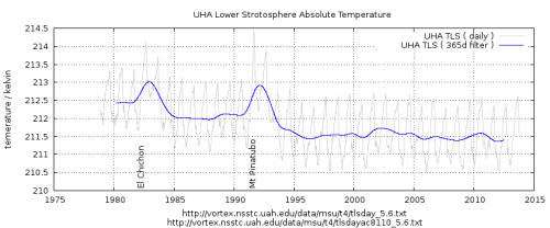 Figure 3 showing changes in lower stratosphere temperature due to volcanism. (Click to enlarge)
A detailed study on the atmospheric physics and radiative effects of stratospheric aerosols by Lacis, Hansen & Sato [2] suggested that radiative forcing at the tropopause can be estimated by multiplying optical depth by a factor of 30 W / m2.
This value provides a reasonably close match to the initial change in ERBE TOA flux. However, later studies[3], [4] , attempting to reconcile climate model output with the surface temperature record have reduced the estimated magnitude of the effect stratospheric aerosols. With the latter adjustments, the initial effect on net TOA flux is notably greater than the calculated forcing, which is problematic; especially since Lacis et al reported that the initial cooling may be masked by the warming effect of larger particles ( > 1µm ). Indeed, in order for the calculated aerosol forcing to be as large as the initial changes in TOA flux, without invoking negative feedbacks, it is necessary to use a scaling of around 40 W/m2. A comparison of these values is shown in figure 4.
What is significant is that from just a few months after the eruption, the disturbance in TOA flux is consistently less than the volcanic forcing. This is evidence of a strong negative feedback in the tropical climate system acting to counter the volcanic perturbation. Just over a year after the eruption, it has fully corrected the radiation imbalance despite the disturbance in AOD still being at about 50% of its peak value. The net TOA reaction then remains positive until the “super” El Nino of 1998. This is still the case with reduced forcing values of Hansen et al as can also be seen in figure 4.

Figure 4 comparing volcanic of net TOA flux to various estimations aerosol forcing. ( Click to enlarge )
The fact that the climate is dominated by negative feedbacks is not controversial since this is a pre-requisite for overall system stability. The main stabilising feedback is the Planck response ( about 3.3 W/m2/K at typical ambient temperatures ). Other feedbacks will increase or decrease the net feedback around this base-line value. Where IPCC reports refer to net feedbacks being positive or negative, it is relative to this value. The true net feedback will always be negative.
It is clear that the climate system takes some time to respond to initial atmospheric changes. It has been pointed out that to correctly compare changes in radiative input to surface temperatures some kind of lag-correlation analysis is required : Spencer & Braswell 2011[5], Lindzen & Choi 2011[6] Trenberth et al 2010 [7]. All three show that correlation peaks with the temperature anomaly leading the change in radiation by about three months.

Figure 5 showing climate feedback response to Mt Pinatubo eruption. Volcanic forcing per Lacis et al. ( Click to enlarge )
After a few months, negative feedbacks begin to have a notable impact and the TOA flux anomaly declines more rapidly than the reduction in AOD. It is quickly apparent that a simple, fixed temporal lag is not an appropriate way to compare the aerosol forcing to its effects on the climate system.
The simplest physical response of a system to a disturbance would be a linear relaxation model, or “regression to the equilibrium”, where for a deviation of a variable X from its equilibrium value, there is a restoring action that is proportional to the magnitude of that deviation. The more it is out of equilibrium the quicker its rate of return. This kind of model is common in climatology and is central of the concept of climate sensitivity to changes in various climate “forcings”.
dX/dt= -k*X ; where k is a constant of proportionality.
The solution of this equation for an infinitesimally short impulse disturbance is a decaying exponential. This is called the impulse response of the system. The response to any change in the input can found by its convolution with this impulse response. This can be calculated quite simply since it is effectively a weighted running average calculation. It can also be found by algebraic solution of the ordinary differential equation if the input can be described by an analytic function. This is the method that was adopted in Douglass & Knox 2005 [17] comparing AOD to lower tropospheric temperature ( TLT ).
The effect of this kind of system response is a time lag as well as a degree of low-pass filtering which reduces the peak and produces a change in the profile of the time series, compared to that of the input forcing. In this context linear regression of the output and input is not physically meaningful and will give a seriously erroneous value of the presumed linear relationship.
The speed of the response is characterised by a constant parameter in the exponential function, often referred to as the ‘time-constant’ of the reaction. Once the time-constant parameter has been determined, the time-series of the system response can be calculated from the time-series of the forcing.
Here, the variation of the tropical climate is compared with a linear relaxation response to the volcanic forcing. The magnitude and time-constant constitute two free parameters and are found to provide a good match between the model and data. This is not surprising since any deviation from equilibrium in surface temperature will produce a change in the long-wave Planck radiation to oppose it. The radiative Planck feedback is the major negative feedback that ensures the general stability of the Earth’s climate. While the Planck feedback is proportional to the fourth power of the absolute temperature, it can be approximated as linear for small changes around typical ambient temperatures of about 300 kelvin. This is effectively a “single slab” ocean model but this is sufficient since diffusion into deeper water below the thermocline is minimal on this time scale. This was discussed in Douglass & Knox’s reply to Robock[18]
It is this delayed response curve that needs to be compared to changes in surface temperature in a regression analysis. Regressing the temperature change against the change in radiation is not physically meaningful unless the system can be assumed to equilibrate much faster than the period of the transient being studied, ie. on a time scale of a month or less. This is clearly not the case, yet many studies have been published which do precisely this, or worse multivariate regression, which compounds the problem. Santer et al 2014 [8], Trenberth et al 2010 [7], Dessler 2010 b [9], Dessler 2011 [10] Curiously, Douglass & Knox [17] initially calculate the relaxation response to AOD forcing and appropriately regress this against TLT but later in the same paper regress AOD directly against TLT and thus find an AOD scaling factor in agreement with the more recent Hansen estimations. This apparent inconsistency in their method confirms the origin of the lower estimations of the volcanic forcing.
The need to account for the fully developed response can be seen in figure 6. The thermal inertia of the ocean mixed layer integrates the instantaneous volcanic forcing as well as the effects of any climate feedbacks. This results in a lower, broader and delayed time series. As shown above, in a situation dominated by the Planck and other radiative feedbacks, this can be simply modelled with an exponential convolution. There is a delay due to the thermal inertia of the ocean mixed layer but this is not a simple fixed time delay. The relaxation to equilibrium response introduces a frequency dependent phase delay that changes the profile of the time series. Simply shifting the volcanic forcing forward by about a year would line up the “bumps” but not match the profile of the two variables. Therefore neither simple regression nor a lagged regression will correctly associate the two variables: the differences in the temporal evolution of the two would lead to a lower correlation and hence a reduced regression result leading to incorrect scaling of the two quantities.
Santer et al 2014 attempts to remove ENSO and volcanic signals by a novel iterative regression technique. A detailed account, provided in the supplementary information[8b], reports a residual artefact of the volcanic signal.
The modelled and observed tropospheric temperature residuals after removal of ENSO and volcano signals, τ , are characterized by two small maxima. These maxima occur roughly 1-2 years after the peak cooling caused by El Chichon and Pinatubo cooling signals.
Figure XXX. Santer et al 2014 supplementary figure 3 ( panel D )
“ENSO and volcano signals removed”

This description matches the period starting in mid-1992, shown in figure 6 below, where the climate response is greater than the forcing. It peaks about 1.5 years after the peak in AOD, as described. Their supplementary fig.3 shows a very clear dip and later peak following Pinatubo. This corresponds to the difference between the forcing and the correctly calculated climate response shown in fig. 6. Similarly, the 1997-98 El Nino is clearly visible in the graph of observational data (not reproduced here) labeled “ENSO and volcano signals removed”. This failure to recognise the correct nature and timing of the volcanic signal leads to an incorrect regression analysis, incomplete removal and presumably incorrect scaling of the other regression variables in the iterative process. This is likely to lead to spurious attributions and incorrect conclusions.

Figure 6 showing tropical feedback as relaxation response to volcanic aerosol forcing ( pre-eruption cycle removed) ( Click to enlarge )
The delayed climatic response to radiative change corresponds to the negative quadrant in figure 3b of Spencer and Braswell (2011) [5] excerpted below, where temperature lags radiative change. It shows the peak temperature response lagging around 12 months behind the radiative change. The timing of this peak is in close agreement with TOA response in figure 6 above, despite SB11 being derived from later CERES ( Clouds and the Earth’s Radiant Energy System ) satellite data from the post-2000 period with negligible volcanism.
This emphasises that the value for the correlation in the SB11 graph will be under-estimated, as pointed out by the authors:
Diagnosis of feedback cannot easily be made in such situations, because the radiative forcing decorrelates the co-variations between temperature and radiative flux.
The present analysis attempts to address that problem by analysing the fully developed response.

Figure 7. Lagged-correlation plot of post-2000 CERES data from Spencer & Braswell 2011. (Negative lag: radiation change leads temperature change.)
The equation of the relationship of the climate response : ( TOA net flux anomaly – volcanic forcing ) being proportional to an exponential regression of AOD, is re-arranged to enable an empirical estimation of the scaling factor by linear regression.
TOA -VF * AOD = -VF * k * exp_AOD eqn. 1
-TOA = VF * ( AOD – k * exp_AOD ) eqn. 2
VF is the volcanic scaling factor to convert ( positive ) AOD into a radiation flux anomaly in W/m2. The exp_AOD term is the exponential convolution of the AOD data, a function of the time-constant tau, whose value is also to be estimated from the data. This exp_AOD quantity is multiplied by a constant of proportionality, k. Since TOA net flux is conventionally given as positive downwards, it is negated in equation 2 to give a positive VF comparable to the values given by Lacis, Hansen, etc.
Average pre-eruption TOA flux was taken as the zero for TOA anomaly and, since the pre-eruption AOD was also very small, no constant term was included.
Since the relaxation response effectively filters out ( integrates ) much of high frequency variability giving a less noisy series, this was taken as the independent variable for regression. This choice acts to minimise regression dilution due to the presence of measurement error and non-linear variability in the independent variable.
Regression dilution is an important and pervasive problem that is often overlooked in published work in climatology, notably in attempts to derive an estimation of climate sensitivity from temperature and radiation measurements and from climate model output. Santer et al 2014, Trenberth et al 2010, Dessler 2011, Dessler 2010b, Spencer & Braswell 2011.
The convention of choosing temperature as the independent variable will lead to spuriously high sensitivity estimations. This was briefly discussed in the appendix of Forster & Gregory 2006 [11] , though ignored in the conclusions of the paper.
It has been suggested that a technique based on total least squares regression or bisector least squares regression gives a better fit, when errors in the data are uncharacterized (Isobe et al. 1990). For example, for 1985–96 both of these methods suggest YNET of around 3.5 +/- 2.0 W m-2 K-1 (a 0.7–2.4 K equilibrium surface temperature increase for 2 ϫ CO2), and this should be compared to our 1.0–3.6 K range quoted in the conclusions of the paper.
Regression results were thus examined for residual correlation.
Results
Taking the TOA flux, less the volcanic forcing, to represent the climatic reaction to the eruption, gives a response that peaks about twelve months after the eruption, when the stratospheric aerosol load is still at about 50% of its peak value. This implies a strong negative feedback is actively countering the volcanic disturbance.
This delay in the response, due to thermal inertia in the system, also produces an extended period during which the direct volcanic effects are falling and the climate reaction is thus greater than the forcing. This results in a recovery period, during which there is an excess of incoming radiation compared to the pre-eruption period which, to an as yet undetermined degree, recovers the energy deficit accumulated during the first year when the volcanic forcing was stronger than the developing feedback. This presumably also accounts for at least part of the post eruption maxima noted in the residuals of Santer et al 2014.
Thus if the lagged nature of the climate response is ignored and direct linear regression between climate variables and optical depth are conducted, the later extended period of warming may be spuriously attributed to some other factor. This represents a fundamental flaw in multivariate regression studies such as Foster & Rahmstorf 2013 [12] and Santer et al 2014 [8] , among others, that could lead to seriously erroneous conclusions about the relative contributions of the various regression variables.
For the case where the pre-eruption variation is assumed to continue to underlie the ensuing reaction to the volcanic forcing, the ratio of the relaxation response to the aerosol forcing is found to be 0.86 +/- 0.07%, with a time constant of 8 months. This corresponds to the value reported in Douglass & Knox 2005 [17] derived from AOD and lower troposphere temperature data. The scaling factor to convert AOD into a flux anomaly was found to be 33 W/m2 +/-11%. With these parameters, the centre line of the remaining 6 month variability ( shown by the gaussian filter ) fits very tightly to the relaxation model.
Figure 6 showing tropical feedback as relaxation response to volcanic aerosol forcing ( pre-eruption cycle removed) ( Click to enlarge )
If the downward trend in the pre-eruption data is ignored (ie its cause is assumed to stop at the instant of the eruption ) the result is very similar ( 0.85 +/-0.09 and 32.4 W/m2 +/- 9% ) but leads to a significantly longer time-constant of 16 months. In this case, the fitted response does not fit nearly as well, as can be seen by comparing figures 6 and 8. The response is over-damped: poorly matching the post-eruption change, indicating that the corresponding time-constant is too long.
 Figure 8 showing tropical climate relaxation response to volcanic aerosol forcing, fitted while ignoring pre-eruption variability. ( Click to enlarge )
The analysis with the pre-eruption cycle subtracted provides a generally flat residual ( figure 9 ), showing that it accounts well for the longer term response to the radiative disruption caused by the eruption.
It is also noted that the truncated peak, resulting from substitution of the mean of the annual cycle to fill the break in the ERBE satellite data, lies very close to the zero residual line.
 Figure 9 showing the residual of the fitted relaxation response from the satellite derived, top-of-troposphere disturbance. ( Click to enlarge )
Since the magnitude of the pre-eruption variability in TOA flux, while smaller, is of the same order as the volcanic forcing and its period similar to that of the duration of the atmospheric disturbance, the time-constant of the derived response is quite sensitive to whether this cycle is removed or not. However, it does not have much impact on the fitted estimation of the scaling factor ( VF ) required to convert AOD into a flux anomaly or the proportion of the exponentially lagged forcing that matches the TOA flux anomaly.
Assuming that whatever was causing this variability stopped at the moment of the eruption seems unreasonable but whether it was as cyclic as it appears to be, or how long that pattern would continue is speculative. However, approximating it as a simple oscillation seems to be more satisfactory than ignoring it.
In either case, there is a strong support here for values close to the original Lacis et al 1992 calculations of volcanic forcing that were derived from physics-based analysis of observational data, as opposed to later attempts to reconcile the output of general circulation models by re-adjusting physical parameters.
Beyond the initial climate reaction analysed so far, it is noted that the excess incoming flux does not fall to zero. To see this effect more clearly, the deviation of the flux from the chosen pre-eruption reference value is integrated over the full period of the data. The result is shown in figure 10.
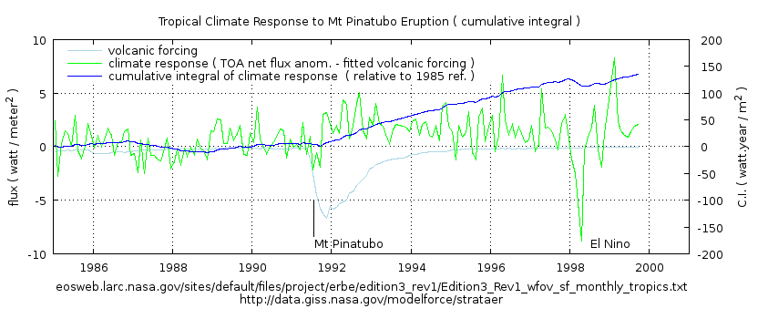 Figure 10 showing the cumulative integral of climate response to Mt Pinatubo eruption. ( Click to enlarge )
Pre-eruption variability produces a cumulative sum initially varying about zero. Two months after the eruption, when it is almost exactly zero, there is a sudden change as the climate reacts to the drop in energy entering the troposphere. From this point onwards there is an ever increasing amount of additional energy accumulating in the tropical lower climate system. With the exception of a small drop, apparently in reaction to the 1998 ‘super’ El Nino, this tendency continues to the end of the data.
While the simple relaxation model seems to adequately explain the initial four years following the Mt Pinatubo event, this does not explain it settling to a higher level.
Discussion
Concerning the more recent estimations of aerosol forcing, it should be noted that there is a strong commonality of authors in the papers cited here, so rather than being the work of conflicting groups, the more recent weightings reflect the result of a change of approach: from direct physical modelling of the aerosol forcing in the 1992 paper, to the later attempts to reconcile general circulation model (GCM) output by altering the input parameters.
From Hansen et al 2002 [4] ( Emphasis added. )
Abstract:
We illustrate the global response to these forcings for the SI2000 model with specified sea surface temperature and with a simple Q-flux ocean, thus helping to characterize the efficacy of each forcing. The model yields good agreement with observed global temperature change and heat storage in the ocean. This agreement does not yield an improved assessment of climate sensitivity or a confirmation of the net climate forcing because of possible compensations with opposite changes of these quantities. Nevertheless, the results imply that observed global temperature change during the past 50 years is primarily a response to radiative forcings.
Form section 2.2.2. Radiative forcing:
Even with the aerosol properties known, there is uncertainty in their climate forcing. Using our SI2000 climate model to calculate the adjusted forcing for a globally uniform stratospheric aerosol layer with optical depth t = 0.1 at wavelength l = 0.55 mm yields a forcing of 2.1 W/m2 , and thus we infer that for small optical depths
Fa (W/m2) ~ 21 tau
…..
In our earlier 9-layer model stratospheric warming after El Chichon and Pinatubo was about half of observed values (Figure 5 of F-C), while the stratospheric warming in our current model exceeds observations, as shown below.
As the authors point out, it all depends heavily upon the assumptions made about size distribution of the aerosols used when interpreting the raw data. In fact the newer estimation is shown, in figure 5a of the paper, to be about twice the observed values following Pinatubo and El Chichon . It is unclear why this is any better than half observed values in their earlier work. Clearly the attributions are still highly uncertain and the declared uncertainty of +/-15% appears optimistic.
3.3. Model Sensitivity
The bottom line is that, although there has been some
narrowing of the range of climate sensitivities that emerge from realistic models [Del Genio and Wolf, 2000], models still can be made to yield a wide range of sensitivities by altering model parameterizations.
If the volcanic aerosol forcing is underestimated, other model parameters will have to be adjusted to produce a higher sensitivity. It is likely that the massive overshoot in the model response of TLS is an indication of this situation. It would appear that a better estimation lies between these two extremes. Possibly around 25 W/m2.
The present study examines the largest and most rapid changes in radiative forcing in the period for which detailed satellite observations are available. The aim is to estimate the aerosol forcing and the timing of the tropical climate response. It is thus not encumbered by trying to optimise estimations of a range climate metrics over half a century by experimental adjustment of a multitude of “parameters”.
The result is in agreement with the earlier estimation of Lacis et al.
A clue to the continued excess over the pre-eruption conditions can be found in the temperature of the lower stratosphere, shown in figure 3. Here too, the initial disturbance seems to have stabilised by early 1995 but there is a definitive step change from pre-eruption conditions.
Noting the complementary nature of the effects of impurities in the stratosphere on TLS and the lower climate system, this drop in TLS may be expected to be accompanied by an increase in the amount of incoming radiation penetrating into the troposphere. This is in agreement with the cumulative integral shown in figure 10 and the southern hemisphere sea temperatures shown in figure 12.
NASA Earth Observatory report [13] that after Mt Pinatubo, there was a 5% to 8% drop in stratospheric ozone. Presumably a similar removal happened after El Chichon in 1982 which saw an almost identical reduction in TLS.
Whether this is, in fact, the cause or whether other radiation blocking aerosols were flushed out along with the volcanic emissions, the effect seems clear and consistent and quite specifically linked to the eruption event. This is witnessed in both the stratospheric and tropical tropospheric data. Neither effect is attributable to the steadily increasing GHG forcing which did not record a step change in September 1991.
This raises yet another possibility for false attribution in multivariate regression studies and in attempts to arbitrarily manipulate GCM input parameters to engineer a similarity with the recent surface temperature records.
With the fitted scaling factor showing the change in tropical TOA net flux matches 85% of the tropical AOD forcing, the remaining 15% must be dispersed elsewhere within the climate system. That means either storage in deeper waters and/or changes in the horizontal energy budget, ie. interaction with extra-tropical regions.
Since the model fits the data very closely, the residual 15% will have the same time dependency profile as the 85%, so these tropical/ex-tropical variations can also be seen as part of the climate response to the volcanic disturbance. ie. the excess in horizontal net flux, occurring beyond 12 months after the event, is also supporting restoration of the energy deficit in extra-tropical regions by exporting heat energy. Since the major ocean gyres bring cooler temperate waters into the eastern parts of tropics in both hemispheres and export warmer waters at their western extents, this is probably a major vector of this variation in heat transportation as are changes in atmospheric processes like Hadley convection.
Extra-tropical regions were previously found to be more sensitive to radiative imbalance that the tropics [link] Thus the remaining 15% may simply be the more stable tropical climate acting as a buffer and exerting a thermally stabilising influence on extra-tropical regions.
After the particulate matter and aerosols have dropped out there is also a long-term depletion of stratospheric ozone ( 5 to 8% less after Pinatubo ) [13]. Thompson & Solomon (2008) [14] examined how lower stratosphere temperature correlated with changes in ozone concentration and found that in addition to the initial warming caused by volcanic aerosols, TLS showed a notable ozone related cooling that persisted until 2003. They note that this is correlation study and do not imply causation.

Figure 11. Part of fig.2 from Thompson & Solomon 2008 showing the relationship of ozone and TLS.
A more recent paper by Soloman [15] concluded roughly equal, low level aerosol forcing existed before Mt Pinatubo and again since 2000, similarly implying a small additional warming due to lower aerosols in the decade following the eruption.
Several independent data sets show that stratospheric aerosols have increased in abundance since 2000. Near-global satellite aerosol data imply a negative radiative forcing due to stratospheric aerosol changes over this period of about -0.1 watt per square meter, reducing the recent global warming that would otherwise have occurred. Observations from earlier periods are limited but suggest an additional negative radiative forcing of about -0.1 watt per square meter from 1960 to 1990.
The values for volcanic aerosol forcing derived here being in agreement with the physics-based assessments of Lacis et al. imply much stronger negative feedbacks must be in operation in the tropics than those resulting from the currently used model “parameterisations” and the much weaker AOD scaling factor.
These two results indicate that secondary effects of volcanism may have actually contributed to the late 20th century warming. This, along with the absence of any major eruptions since Mt Pinatubo, could go a long way to explaining the discrepancy between climate models and the relative stability of observational temperatures measurements since the turn of the century.
Once the nature of the signal has been recognised in the much less noisy stratospheric record, a similar variability can be found to exist in southern hemisphere sea surface temperatures. The slower rise in SST being accounted for by the much larger thermal inertia of the ocean mixed layer. Taking TLS as an indication of the end of the negative volcancic forcing and beginning of the additional warming forcing, the apparent relaxation to a new equilibrium takes 3 to 4 years. Regarding this approximately as the 95% settling of three times-constant intervals ( e-folding time ) would be consistent with a time constant of between 12 and 16 months for extra-tropical southern hemisphere oceans.
These figures are far shorter than values cited in Santer 2014 ranging from 30 to 40 months which are said to characterise the behaviour of high sensitivity models and correspond to typical IPCC values of climate sensitivity. It is equally noted from lag regression plots in S&B 2011 and Trenberth that climate models are far removed from observational data in terms of producing correct temporal relationships of radiative forcing and temperature.

Figure 12. Comparing SH sea surface temperatures to lower troposphere temperature.
Though the initial effects are dominated by the relaxation response to the aerosol forcing, both figures 9 and 12 show a additional climate reaction has a significant effect later. This appears to be linked to ozone concentration and/or a reduction in other atmospheric aerosols. While these changes are clearly triggered by the eruptions, they should not be considered part of the “feedback” in the sense of the relaxation response fitted here. These effects will act in the same sense as direct radiative feedback and shorten the time-constant by causing a faster recovery. However, the settling time of extra-tropical SST to the combined changes in forcing indicates a time constant ( and hence climate sensitivity ) well short of the figures produced by analysing climate model behaviour reported in Santer et al 2014 [8].
IPCC on Clouds and Aerosols:
IPCC AR5 WG1 Full Report Jan 2014 : Chapter 7 Clouds and Aerosols:
No robust mechanisms contribute negative feedback.
7.3.4.2
The responses of other cloud types, such as those associated with deep convection, are not well determined.
7.4.4.2
Satellite remote sensing suggests that aerosol-related invigoration of deep convective clouds may generate more extensive anvils that radiate at cooler temperatures, are optically thinner, and generate a positive contribution to ERFaci (Koren et al., 2010b). The global influence on ERFaci is
unclear.
Emphasis added.
WG1 are arguing from a position of self-declared ignorance on this critical aspect of how the climate system reacts to changes in radiative forcing. It is unclear how they can declare confidence levels of 95%, based on such an admittedly poor level of understanding of the key physical processes.
Conclusion
Analysis of satellite radiation measurements allows an assessment of the system response to changes in radiative forcing. This provides an estimation of the aerosol forcing that is in agreement with the range of physics-based calculations presented by Lacis et al in 1992 and is thus brings into question the much lower values currently used in GCM simulations.
The considerably higher values of aerosol forcing found here and in Lacis et al imply the presence of notably stronger negative feedbacks in tropical climate and hence imply a much lower range of sensitivity to radiative forcing than those currently used in the models.
The significant lag and ensuing post-eruption recovery period underlines the inadequacy of simple linear regression and multivariate regression in assessing the magnitude of various climate ‘forcings’ and their respective climate sensitivities. Use of such methods will suffer from regression dilution, omitted variable bias and can lead to seriously erroneous attributions.
Both the TLS cooling and the energy budget analysis presented here, imply a lasting warming effect on surface temperatures triggered by the Mt Pinatubo event. Unless these secondary effects are recognised, their mechanisms understood and correctly modelled, there is a strong likelihood of this warming being spuriously attributed to some other cause such as AGW.
When attempting to tune model parameters to reproduce the late 20th century climate record, an incorrectly small scaling of volcanic forcing, leading to a spuriously high sensitivity, will need to be counter-balanced by some other variable. This is commonly a spuriously high greenhouse effect, amplified by presumed positive feedbacks from other climate variables, less well constrained by observation ( such as water vapour and cloud ). In the presence of the substantial internal variability, this can be made to roughly match the data while both forcings are present ( pre-2000 ). However, in the absence of significant volcanism there will be a steadily increasing divergence. The erroneous attribution problem, along with the absence of any major eruptions since Mt Pinatubo, could explain much of the discrepancy between climate models and the relative stability of observational temperature measurements since the turn of the century.
[Notes] Data, Supplementary Information
References:
[1] Self et al 1995
“The Atmospheric Impact of the 1991 Mount Pinatubo Eruption”
http://pubs.usgs.gov/pinatubo/self/
[2] Lacis et al 1992 : “Climate Forcing by Stratospheric Aerosols
Click to access 1992_Lacis_etal_1.pdf
[3] Hansen et al 1997 “Forcing and Chaos in interannual to decadal climate change”
Click to access Hansen_etal_1997b.pdf
[4] Hansen et al 2002 : “Climate forcings in Goddard Institute for Space Studies SI2000 simulations”
Click to access hansen_etal_2002.pdf
[5] Spencer & Braswell 2011: “On the Misdiagnosis of Surface Temperature Feedbacks from Variations in Earth’s Radiant Energy Balance”
http://www.mdpi.com/2072-4292/3/8/1603/pdf
[6] Lindzen & Choi 2011: “On the Observational Determination of Climate Sensitivity and Its Implications”
Click to access 236-Lindzen-Choi-2011.pdf
[7] Trenberth et al 2010: “Relationships between tropical sea surface temperature and topâ€ofâ€atmosphere radiation”
http://www.mdpi.com/2072-4292/3/9/2051/pdf
[8] Santer et al 2014: “Volcanic contribution to decadal changes in tropospheric temperature”
http://www.nature.com/ngeo/journal/v7/n3/full/ngeo2098.html
[8b] Supplementary Information:
Click to access ngeo2098-s1.pdf
[9] Dessler 2010 b “A Determination of the Cloud Feedback from Climate Variations over the Past Decadeâ€
Click to access dessler10b.pdf
[10] Dessler 2011 “Cloud variations and the Earth’s energy budgetâ€
Click to access Dessler2011.pdf
[11]Forster & Gregory 2006
“The Climate Sensitivity and Its Components Diagnosed from Earth Radiation Budget Dataâ€
Click to access Forster_sensitivity.pdf
[12] Foster and Rahmstorf 2011: “Global temperature evolution 1979-2010”
http://stacks.iop.org/ERL/6/044022
[13] NASA Earth Observatory
http://earthobservatory.nasa.gov/Features/Volcano/
[14] Thompson & Soloman 2008: “Understanding Recent Stratospheric Climate Change”
http://journals.ametsoc.org/doi/abs/10.1175/2008JCLI2482.1
[15] Susan Soloman 2011: “The Persistently Variable “Background†Stratospheric Aerosol Layer and Global Climate Change”
http://www.sciencemag.org/content/333/6044/866
[16] Trenberth 2002: “Changes in Tropical Clouds and Radiation”
[17] Douglass & Knox 2005: “Climate forcing by the volcanic eruption of Mount Pinatubo”
Click to access 2004GL022119_Pinatubo.pdf
[18] Douglass & Knox 2005b: “Reply to comment by A. Robock on ‘‘Climate forcing by the volcanic eruption of Mount Pinatubo’’”
Click to access reply_Robock_2005GL023829.pdf
Biosketch: Greg Goodman has a degree in applied physics, professional experience in spectroscopy, electronics and software engineering, including 3-D
computer modelling of scattering of e-m radiation in the Earth’s atmosphere. Previous posts by Greg Goodman:
- Interdecadal in Northern Hemispheric Sea Ice
- On the adjustments to the HADSST3 data set
- Data ‘corruption’ by running mean smoothers
JC note: This is a guest post, that was submitted via email. As with all guest posts, please keep your comments civil and relevant.

A bombshell hit.
High latitude volcanoes are very productive, Icelandic had only 2% of the world eruptions since 1600, but released 30% of the global tephra.
– In short term reduction of temperature (as per all known reasons)
– Most of the ash is eventually deposited on the Arctic ice, increasing the albedo and speeding the surface ice and snow melt. There is also effect of mineral content reducing freezing and melting temperatures.
Conclusion is that sub-arctic region volcanoes are contributing more to global warming than cooling.
http://www.vukcevic.talktalk.net/CRUTEM4.gif
It is important that there is a correlation and possible link of polar auroral region volcanic eruptions and the collar activity as discussed here and in the subsequent comment
auto correct typo:
correlation and possible link of the polar auroral region volcanic eruptions and solar activity
vuk
Thanks for reference to tephra. That is a new word for me. Two questions. What is it about the Iceland volcanoes that allows 2% of the eruptions to emit 30% of the tephra and if it is the amount from 1600 what kind of methods were used to determine those amounts for the 2% and the 30%. Thanks.
Vuk
I was just wonderin, doesn’t volcanic ash, settled upon arctic ice, decrease the albedo of the arctic ice?
Hi
1. Iceland is an island created by magma (high basalt content) pouring out between separating plates. Subduction areas volcanoes are result of sinking and melting of the crust, thus amount of magma expelled is dependent the amount of sinking material.
http://www.ecomapcostarica.com/ref/volcano/subduction.png
2. Solidified lava is easily dated; I suppose geologists use subsequent layers area and volume calculations. I often see quoted ‘x or y km3’ of lava for centuries or even millennia old eruptions. Vesuvius (of Pompeii infamy 79AD) is quoted as 9 km3 of pumice.
Justin, thanks. it was a slip-up, but from the rest of the sentence it is clear what is meant. (blogging a lot today, mostly on WUWT).
it should be:
… ash is eventually deposited on the Arctic ice decreasing the albedo and speeding the surface ice and snow melt.
Albedo is a measure of the “whiteness” of a surface, black = 0, white = 1.
I need to read what I write..
Vuk,
Surely the productivity of Icelandic volcanoes is due to their geological structure, not the latitude at which they are sited? (Just to clarify)
Mr. Abbot
Yes, agree, the opening sentence should have been better phrased. It was meant to differentiate immediately from the article’s ‘tropical’ subject, but hopefully the reason was clarified by the answer to ceresco kid.
Circular in a spiraling, swirling, flushing sort of way;
Regression dilution by Charybditic Bay.
H/t for the first line to commenter hunter speaking of Marotzke and Forster at ClimateAudit.
============
They just wanted to show how statistics are not supposed to be done and didn’t realize Nature would take their paper seriously.
Question Why are lunar-solar influences — which figured prominently in Goodman’s 2013 analysis “On Zen and the Art of Climate Analysis“ — entirely disregarded in this 2015 Goodman analysis (as far as FOMD can tell)?
Concern Will volcanic influences too be entirely disregarded in some forthcoming 2017 Goodman analysis? What prevents wholly new statistical models from being generated every two years … with each new model having zero connection to previous models.
Such past-forgetful modeling ain’t science … is it?
Conclusion Statistical analyses (no matter how ingenious) aren’t worth much, unless they are disciplined by thermodynamic considerations, paleo data, large-scale climate models … and by acknowledgement and incorporation of prior statistical models.
I originally ignored this stupid comment as an obvois troll. However, for the record I’ll point out what Fanny is stupidly missing.
The previous article he refers was looking at decadal scale lunar cycles and thier relation to detection of 11y solar cycles.
The peak volcanic response has a lag of about 12mo. That’s an order of magnitude faster the luni-solar and so does not contradict or invalidate the main analysis here.
Ideally all these things need to be combined, since there may be some cross-over. But unless some attempt is made to isolate and identify them individually, putting them all in a box and shaking it very hard is not going to give the right answer.
Greg: I have only had time to skim this so apologies if I have missed something vital, but I think you are saying that the late 20th C warming was ‘juiced’ by volcanoes. In which case why has the temperature not gone back down since Mt Pintubo? Presumably there is AGW compensating and keeping the temperature high? And what value do you favour for climate sensitivity?
The indications are that the secondary effects of the eruptions introduced a supplementary radiative forcing, not a temporary warming. This does rule out the presence of some AGW but does mean that unless this process is recognised and properly understood it will almost certainly get erroneously attrubuted to AGW.
There are the other issues I raised such as not regressing the correct form a radiative forcing and regression dilution. There are a lot of papers getting through peer review that do not even the basics. right. Using linear regression with large errors in the x variable is probably the most basic and widespread.
Greg,
Is this what you meant? “This does rule out the presence of some AGW but does mean that unless this process is recognised and properly understood it will almost certainly get erroneously attrubuted to AGW.” I assume you left out “not.”
Indeed, thanks for spotting that.
I wonder at the Maunder,
A hulkin’, bulkin’ vulcan yonder,
Or is it this, Ol’ Sol to ponder?
===================
” When attempting to tune model parameters to reproduce the late 20th century climate record, an incorrectly small scaling of volcanic forcing, leading to a spuriously high sensitivity, will need to be counter-balanced by some other variable. … ”
32 virgin free variables. Are we in Paradise? or the other place?
Even if humanity arguably does have some minor impact on the global temperature of the Earth it is estimated that about half of the effect will occur over the next 100 years and is likely to be a good thing (e.g., fewer natural disasters and less poverty) while, “the equilibrium temperature response [caused by the remaining effect] may not be attained for several millennia.” Our schoolteachers aren’t really alarmed about the weather in 4015: they are scared today about something that hasn’t happened. (See current research –e.g., Monckton, et al, below — Why models run hot: results from an irreducibly simple climate model — which shows, “the now-realized projections of the general-circulation models have proven to be relentlessly exaggerated.” )
Wag,
Wrong (I learned this from you know who). Humans are the main driver of climate, modifying the climate to suit our bathing. It’s gonna get hot HOT, I say, and the seas are gonna rise way up. Don’t believe me? Waterfront property is dirt cheap now and headed down. You can’t even give away a Malibu beach house. Poor Barbara S., she has a stranded sand asset. There should be government grants for people with soon to be drowned beach mansions. Oh, the humanity…
I am not sure that your charts show the Pinatubo response timing all that well. Tropical oceans have an inconsistent seasonal cycle that impacts thermal inertia making it look like Pinatutubo response started a half year before the eruption. If you just remove seasonal cycle with anomaly you can throw off the relationship.
http://redneckphysics.blogspot.com/2015/02/tropical-ocean-and-stratosphere.html
The stratosphere also has seasonal “tidal” fluctuations.
I know the article is a bit long but I suggest you read it before trying to comment. In particular the preceding downward trend is discussed and some attempt to account for this is made. In fig 4 the timing issue you raise is no longer present.
http://climategrog.files.wordpress.com/2014/04/erbe_vs_aerosol_forcing1.png?w=843
Right, that one has peak forcing about 5 months after the event and peak response a month or so earlier.
The stratosphere has peak response about a year and a half after the event.
http://1.bp.blogspot.com/-rrG5jfTHR8I/VNTeamG2i8I/AAAAAAAAMi4/P5Aeo18ZxPQ/s1600/tropical%2BSSE%2Band%2BLS%2BTenlarged.png
“Right, that one has peak forcing about 5 months after the event and peak response a month or so earlier. ”
Fig 4 does not even show the response. I’m more that willing to discuss any relevant criticism but please read and understand the article rather than posting from the hip.
Then let’s get our terminology together, Figure 4 has TOA net dropping to a minimum about 3-4 months after the event and the standard forcing estimate at a minimum about 5 months after the event.
In figure 10 you call that a climate response after ignoring the pre-eruption down trend which I believe is best not ignore since it appears to be “tidal” related to annual solar variation and would be lost when converting to anomaly.
I am sure your paper is absolutely bullet proof, but if there is a reason for the pre-eruption down turn why ignore it?
Yes, please do get the terninology right. Or at least read what is on the graphs before trying to comment. Fig 10 does not show the same thing as fig4, This is not trivial, so if you wish to comment, for a third time I invite you read before posting a comment.
You are technically competent so if you took the time to understand rather than sniping, you may be able to come up with a valid criticism. That would certainly be of value.
Greg, I think PaulK has the jargon down better. I wasn’t sniping as much as curious. I personally look at weakly damped response instead of relaxation, because that would produce the decreasing oscillations in higher inertia response and increasing in lower inertia response, but you are comparing to sop methods.
Thanks Capt.
What do you propose is doing the damping? It seems hard not to have something like a relaxation because of strong Planck feedback.
True it should be non linear if being more rigorous but that would just give sharper than linear relaxation and probably some overshoot.
Looking at my last graph, there may be some mileage in that idea.
There would still seem to be some additional forcing introduced after the events, since even with non-linear and overshoot it should still settle to its pre-eruption level. Last fig shows both TLS and SST taking a lasting offset from initial conditions.
Greg, “What do you propose is doing the damping?”
I am looking at clouds/convective triggering. Not all that easy, but about the best shot I see. In the tropics convective triggering kicks in between 27 and 28 C.
I think I discussed this below in reply to Judith’s comment about the Emanuel paper. Even quite complex local behaviour can end up being simple negative feedback when viewed on a larger scale, not individual storms. The internal +ve feedbacks make it a strong, non linear -ve feedback effect. That is probably consistent with the bifurcation that Emanuel is describing.
This again ties in with the idea of something more reactive than a simple relaxation that could produce the kind of overshoot seen in my last figure in the article.
This could be some other internal variability but could also be overshoot from a non linear neg. f/b.
Greg, It is pretty interesting.
https://lh4.googleusercontent.com/-AXHp8YWqd80/VNZ2A0swqQI/AAAAAAAAMls/AwnHS_GPirU/w569-h331-no/with%2Blag%2Bwith%2Bcurve.png
I ran this comparison of SST, LS and OLR lagged by 27 months then did this correlation with SST
https://lh3.googleusercontent.com/-sT1L_Wmi5xk/VNZ2A9vospI/AAAAAAAAMlo/llYwPu2hAzU/w839-h437-no/with%2Blag%2Bcorrelations.png
There is not a lot of difference between ENSO and Pinatubo, so if you remove ENSO you would tend to exaggerate Pinatubo.
Again I suspect tropical SST has reached a convective limit, but the data I have access to has a good many holes. That was trimmed at 2010 because of the OLR data on climate explorer.
The 27 month lag btw is due to tropical SST response to solar, the tide thing I suspect.
I’m not really following what you are doing, could you be more specific?
What is LS? What is a “60mo correlation? I’m familiar the correlation fn where the lag is varied or a correlation with a lag of 60mo which is a single number. I do not understand what you are plotting here.
If you say it’s interesting, I’d like to have enough information to see what it represents.
Also, wrt removing ENSO, many have attempted this but since ENSO is basically tropical SST metric, it does not make sense to subtract it while attempting to look at the effects a change in radiative forcing on surface climate. You’d be trying to remove part of the signal you are supposed to be looking for. People just don’t think. ( eg Santer 2014 )
However, there is a preceding downward trend in SST and other metrics before Mt P. , I did attempt to account for this in the processing in the article.
Greg, “I’m not really following what you are doing, could you be more specific?”
It’s exploring more than anything else. The satellite data starts at an inconvenient period and solar reconstructions are questionable so I am trying to verify lags and timing of ENSO peaks with solar peaks/valleys.
Volcanic response is all over the place so I was hoping that would help with the timing. The main problem I am having is it hard to determine if something is volcanic or related to solar. ENSO seems to mainly be a function of solar.
Greg, let me expand a bit. There aren’t any truly independent data sets prior to the satellite era because the system is so tightly coupled. Using tropical SST, NH land Ts and Solar I am thinking would produce three more independent than not sets to use for timing of past volcanic events.
Kringing and long range interpolation though smears SST and land so that is a bit of a problem.
Thanks Capt. , in trying to cut this down into snippets that would not get blocked I lost this bit. It’s not a case of where are you going but that I just don’t follow what you are plotting since it is not marked clearly enough.
What is LS? What is a “60mo correlation? I’m familiar the correlation fn where the lag is varied or a correlation with a lag of 60mo which is a single number. I do not understand what you are plotting here.
If you say it’s interesting, I’d like to have enough information to see what it represents.
What is LS? What is a “60mo correlation?
the correlation fn
Ah , I get it. ( the moderation lunacy )
someone who is famil-iar is a L_I_A_R and hits a moderation hold.
I’m au fait with the correlation function where the lag is varied, or a correlation with a lag of 60 mo which is a single number. I do not understand what you are plotting here.
Yes, this is why false attribution is so easy and 30 years of simplistic “linear trends” and ignorant regression fitting has not helped one bit.
There is similarity in timing of Mt P , El Chichon and the solar signal. Solar also affects ozone production hence concentration hence SW and volcanism likely affects ENSO. I also suspect that there is a tidal element to ENSO but that’s storey for another day.
The first step is to learn when to do regression ( not on scatter plots with noisy x data ) and to regress physically meaningful quantities, ie don’t regress a radiative flux directly against temperature unless you can show that the system equilibrates quicker than the timing of the main transients in the forcing flux.
Oh I am sorry, LS is lower stratosphere I think you use TLS, but I have converted it to energy anomaly. 60 month correlation is just a sequential correlation of SS”E” or sea surface energy anomaly with LS and the OLR outgoing long wave radiation lagged by 27 months. I used 211.5K as the average LS temperature to produce the energy anomaly. The conversions don’t effect the correlation, but they provide an interesting picture of how tight the energy range is limited.
Greg, “Yes, this is why false attribution is so easy and 30 years of simplistic “linear trends” and ignorant regression fitting has not helped one bit.”
btw, one of the reasons I like sequential correlations is they are a quick and easy test with just a dumb spread sheet. You need to find something more mainstream afterwards, but it is a neat quick and dirty test.
‘
Great post, so much to digest.
And now, time for a little, very little, humor:
So volcanos might actually warm the climate? Do we have to turn the hokey stick upside down?
Sorry, that was low hanging fruit.
Very interesting post. Is it being submitted for publication elsewhere?
Greg Goodman
Thank you for this post. If I got the gist correctly, I have some additional questions if you don’t mind.
If an equatorial volcanic eruption effluent reduces equatorial stratospheric ozone, what is the mechanism?
As a corollary, what produces equatorial stratospheric ozone?
Is there an “ideal” balance of ozone in the equatorial stratosphere? or, is equatorial stratospheric ozone a “control knob?”
what is the mechanism? volcanoes eject large quantities of SO2, this mixes with water vapour and forms diluted sulphuric acid aerosols. As I understand it, this is a catalyst that breaks down ozone. There is literature on that. You will probably find some useful links in the refs and S.I sections which Judith separated out to a separate file ( see link at and of article ).
I make summary explanation of the form of the AOD data as the result of two chemical kinetic processes here and propose it as a physical explanation for Douglass & Knox’s empirical fit.
https://climategrog.wordpress.com/?attachment_id=1278
It would appear that there has been a slow recovery in stratospheric ozone since the period of data studied here from ERBE I would not be surprised if this was not also described by a relaxation to equilibrium but with a time constant probably of the order of 10 years.
This may be one factor contributing to “the pause”.
Greg Goodman,
Correct me if I’m wrong, but ozone is formed in the upper atmosphere by UVC from the Sun. It is extremely reactive, and therefore reforms into O2 almost instantaneously, if it chances upon another oxygen atom, or pretty much anything else.
Your statement that SO2 emananating from volcanos forms a catalyst which breaks down ozone is misleading at best, and mischievous at worst.
Ozone needs no catalyst. It reverts to O2 all by itself, and after absorbing a sufficient amount of UVC – or shorter – more ozone is created.
Am I wrong?
Live well and prosper,
Mike Flynn.
Mike, I think I said the sulphuric acid was the catalyst, not SO2. However, this is probably technically incorrect. A catalyst does not take part in a chemical reaction and is still there afterwards.
Acids are reducing agents, ie they remove oxygen. If you reduce ozone ( O3 ) you get O2.
Even if that is likely to happen anyway a reducing agent is increasing the chances of it happening and thus will lower the equilibrium concentration.
No mischief required.
Greg Goodman,
You wrote –
“Mike, I think I said the sulphuric acid was the catalyst, not SO2. However, this is probably technically incorrect. A catalyst does not take part in a chemical reaction and is still there afterwards.
Acids are reducing agents, ie they remove oxygen. If you reduce ozone ( O3 ) you get O2.
Even if that is likely to happen anyway a reducing agent is increasing the chances of it happening and thus will lower the equilibrium concentration.
No mischief required.”
I point out that I did not say that you said SO2 was the catalyst.
As you acknowledge, your statement about catalysts was technically incorrect. This is supposed to be a technical thread, so technically wrong is wrong – is it not?
Your implication that SO2 products influence the amount of free oxygen or the amount of UVC from the Sun, seems unlikely. Have you any real evidence that this is the case?
If not, then the ozone cycle will proceed as always. In the absence of appropriate radiation, oxygen molecules do not spontaneously form ozone in any meaningful way.
Now as to your statement that H2SO4 reduces O3 to O2, what happens to the spare oxygen atom left over? Does it combine with H2SO4 to form H2SO5? Or possibly with O2 to form ozone, again?
I believe you may be accidentally making stuff up due to excessive enthusiasm.
Your statement –
“Even if that is likely to happen anyway a reducing agent is increasing the chances of it happening and thus will lower the equilibrium concentration.” is an unverified assertion, which appears to have no factual basis.
Obviously, if you are wrong in this small matter, it might lead people to think that your grasp of atmospheric physics is similarly lacking.
Finally, I asked before – Am I wrong?
Your lack of meaningful response provides me with no reason to doubt that I was right.
Live well and prosper,
Mike Flynn.
what happens to the spare oxygen atom left over?
2O₃ → 3O₂
Vaughan Pratt,
Thanks. I know. Greg Goodman said that H2SO4 reduces O3 to O2. I’m with you, I think. O3 needs no sulphuric acid or anything else to revert to O2, and hang about waiting for a bit of UVC, or stronger, to break the molecular bond and create two ferociously reactive oxygen atoms.
And so continues the grand ozone circle. Renewable and inexhaustible, given oxygen and the Sun. A bit like us, really.
Live well and prosper,
Mike Flynn.
“Your statement that SO2 emananating from volcanos forms a catalyst which breaks down ozone is misleading at best, and mischievous at worst.”
Mike, ozone did drop after both Mt P and El Chichon and stayed down. There are at least two refs for that in the article plus the graph from Solomon’s paper. That is not controversial.
If you want to understand more about the exact mechanism I suggest you follow the refs provided or do you own research rather than trying to deny that it happens and suggesting “mischief” on my part.
Mike Flynn,
you seem to have lost interest but for posterity, here is a paper explaining the various processes of SO2 conversion to SO4- and sulphuric acid, with equilibrium reactions. some reference to Pinatubo.
http://www.geos.ed.ac.uk/~dstevens/Presentations/Papers/stevenson_gssp03.pdf
http://volcanoes.usgs.gov/hazards/gas/s02aerosols.php
Ozone depletion promoted by volcanic sulfur aerosols.
The sulfate aerosols also promote complex chemical reactions on their surfaces that alter chlorine and nitrogen chemical species in the stratosphere. This effect, together with increased stratospheric chlorine levels from chlorofluorocarbon (CFC) pollution, generates chlorine monoxide (ClO), which destroys ozone (O3).
From Self et al (ref 1 of the article) “…. approximately 180 days after the eruption and still remained an order of magnitude higher than ambient levels for at least 2 years after the eruption. Such a great enhancement in aerosol mass and surface area due to the eruption produced significant variations of atmospheric optical properties and ozone abundance.”
Mike Flynn: “Your lack of meaningful response provides me with no reason to doubt that I was right.”
Your lack of ability to read even the first reference in the reference list of the article leaves you with the spurious assumption that you are always right and that it is the duty of others to prove this is not the case.
Next time, read first, shoot ( from the mouth ) later.
live long and prosper ;)
Greg Goodman,
I am unsure why you assumed I didn’t read some of your references.
I did. I didn’t see anything to contradict my statements.
When your first reference contains statements such as –
“This ozone decrease may be due in part to the presence of Pinatubo aerosols . . . “, and so on, I do not accept mere apparent correlation as fact.
And so it goes. As I said before, given sufficient O2, and sufficiently energetic radiation, ozone forms. Unless you can either reduce the amount of the available radiation, or the oxygen available for it to interact with, you cannot prevent the formation of ozone.
A short quote, to give you the flavour of some of the complexity associated with measuring ozone levels, is as follows –
“Ozone layer: The percentage of ozone peaks near the top of the stratosphere, and that, in combination with the greater amount of UV at height (less reaches lower altitudes), produces the greatest heating of the middle atmosphere at the stratopause. However, since the amount of air increases rapidly as you go downwards, even though the percentage of ozone is less at lower altitudes, the peak abundance in terms of actual numbers of molecules is greatest in the middle of the stratosphere. As a result, a graph showing the ozone concentration in the atmosphere will peak at the stratopause if it refers to heating by ozone, or ozone concentration; while a graph showing the actual amount of ozone will peak in the middle stratosphere, because the number of ozone molecules must decrease at higher altitudes if only because there is less air of all types at higher altitudes”.
The Professor who wrote this is has degrees in astronomy and physics. The quote also appears to be factual, backed up by atmospheric scientists generally.
There are many myths which enjoy wide circulation, but the thought that there is a danger that the supply of ozone can be exhausted, leading to subsequent frying by exposure to, say, UVC, is pure nonsense. Incoming UVC is absorbed by oxygen and water vapour, for a start. There is plenty of this life giving stuff between us and the Sun.
I always assume I am right. If someone provides facts which demonstrate that I am not, I change my mind. I assume you would do the same, unless you are a Warmist. They seem impervious to facts, preferring assumptions, guesses, strident assertions, and hand waving in general.
If you can adduce any facts – rather than unsupported assertions – to challenge anything relevant that I have said, feel free.
I’m fairly sure you can’t, but I have been wrong before. For example, I didn’t believe antibiotics could cure stomach ulcers. I was wrong.
CO2 does not create energy. It doesn’t trap, store, or accumulate heat in any physically different way to other gases. It can be heated, and it can cool. So can other matter.
Live well and prosper,
Mike Flynn.
Again from Self et at: “….. [stratospheric] temperatures in 1993 were the coldest ever recorded (Christy and Drouilhet, 1994; Monastersky, 1994) and may be related to ozone destruction in the lower stratosphere. Stratospheric temperatures also plummeted and stayed cooler than average for 7 years after the El Chichón eruption.”
IMPACT ON STRATOSPHERIC CHEMISTRY AND OZONE
“Sulfate aerosols in the stratosphere can catalyze heterogeneous reactions that affect global ozone abundance (Farman and others, 1985; Hofmann and Solomon, 1989; Wolff and Mulvaney, 1991; Prather, 1992). These heterogeneous processes occurring on the surface of sulfate particles can convert stable chlorine reservoirs (such as HCl and ClONO2) into photochemically active chlorine species (Cl2, ClNO2, HOCl) that are active in ozone destruction (Hofmann and Solomon, 1989; Solomon and others, 1993). Increase in aerosol surface area due to the Pinatubo volcanic eruption has had a considerable effect on global ozone (Bhartia and others, 1993;”
That was where I formed the (correct) idea this was a catalytic effect. Because unlike Mke Flynn I had read and cited the the relevent literature.
Thanks for you last reply Mike,
The Self paper, which is a meta study, is quite long and contains large number of references to original studies from which it draws. It goes into a lot more depth that the snippet you quoted.
I don’t see anyone suggesting ozone formation was prevented but as I said earlier, if there is an additional process destroying it, it will lower the equilibrium concentration. There was a measured drop of between 5 and 8% as I quoted in the article.
There has been a very gradual recovery in recent years and this may be one factor contributing to “the pause” and the decline in global temps since 2005.
I welcome challenges to what I have done. That was the aim of getting posted on this site, which has, amongst the clowns, a group of highly competent readers.
However, I would appreciate that commenters check the sources I provide to backup my statements and avoid character slurs like suggesting “mischief”.
If you still think that ozone levels should remain constant and are unaffected by the eruption, perhaps you could elaborate on why Self and the many refs he uses and Thompson and Solomon’s paper I also cited are wrong.
The main point is, that there was a clear, step cooling in TLS as the result of both eruptions that can not be accounted for by fitting a “linear trend” and attributing it to AGW.
This implies that there will be a warming effect reflected in surface temps that is not correctly modelled and is leading to false attribution.
Is there any way the magnetosphere can modify the location, particularly the latitude, of vulcanism?
===========
Doubtful. Vulcanism is a function of plate tectonics. There is some literature suggesting tidal forces may affect timing of events. But virtually all volcanos save Hawaii are either on spreading rifts (Iceland) or over subduction zones (US west Coast), locations fixed in time by plate edges (well fixed to within a couple of centimeters/yr tectonic motion. Hawaii sits over a mantle plume hotspot; a ‘hole’ in a Pacific plate.
Rid
“Vulcanism…plate tectonics…”
There are also “hot spots” and LIPs (Large Igneous Province) with implications for climate change and extinctions.
http://en.m.wikipedia.org/wiki/Large_igneous_province
Oops… I meant to type “Rud” but I am fumbling with an iPad, which is a challenge for typing. Also, you mentioned “hot spot”, which I second. :)
Hi Kim
In an extremely remote cases, yes. Strength of the magnetosphere protects the Earth from solar particles impact, of which the coronal mass ejections (CME) ‘proton showers’ are the most intense. These impacts initiate geomagnetic storms in the polar regions, aurora being most visible and pleasant effect, while the more tangible ones could be very damaging, look up Carrington event 1859 or ‘The Day the Sun Brought Darkness’ Quebec 1989. One average two hour long geomagnetic storm releases into auroral (night time) region same energy as M 5.5 earthquake, while many are much stronger and longer. Geomagnetic storm preceding Japan’s March 2011 earthquake and tsunami lasted 14 hours http://www.vukcevic.talktalk.net/Japan.gif
at the time I was monitoring signal on-off, half way through somewhat concerned, I posted a note on WUWT
Since there is an apparent correlation between Ap index (measure of geomagnetic intensity) and auroral volcanic region eruptions, there is remote possibility that a repeated sequence of strong prolonged GM storms may, just may but not necessarily will, trigger a volcano to erupt which was on the verge of erupting anyway.
If correlation indicates causation, than geomagnetic storms are the synchronising rather than a driving force.
Now back to your question:
If the earth’s magnetosphere is half the strength, geomagnetic storms would be 4 times stronger and 4x more efective, and so on. Eventually in the distant future when the earth’s liquid outer core sufficiently cools down, thermal convection may stop, earth will loose its magnetic field, and the solar experts say that most of our atmosphere will be blown away by solar wind. I have a good reason to doubt it, but what is certain is that most living things if still around, will be killed by solar radiation.
We can fill the silent coliseum of ignorance about magnetic effects with the cackling cacaphony of confusion about biotic effects. Yes, let’s have a concert.
==================
Greg
This item was referring to the lifetimes work of Hubert Lamb. Do you agree with it?
—- —-
This painstaking work, using scientific reports from the well-documented eruption of Krakatoa in 1883, and also from Iceland, the Mediterranean, Alaska, Greenland, Kamchatka, and elsewhere, led to his thesis which developed an assessment of the world’s volcanic eruptions since 1500. His paper, ‘Volcanic dust in the atmosphere… A chronology and assessment of its meteorological significance’, was published by the Royal Society in 1970. And with its publication, the Lamb Dust Veil Index entered the scientific literature.
My investigations had shown that beyond reasonable doubt that great volcanic eruptions do affect the weather and climate for several years afterwards, while suspended materials – not only the fine dust, but minute droplets and even gases – thrown up into the atmosphere by the blast are still present. 2
The study showed that it was the greatest explosions in the low latitudes between about 30°N and 30°S that most regularly yield products that spread around the world, and that the most regular effect of such eruptions was a weakening of the strength of the global circulation. Whereas an eruption in the middle and high latitudes tended to strengthen the circulation in that hemisphere.”
——- ——–
tonyb
Hi Tony.
Well the “minute droplets” are the volcanic aerosols that this post is all about. They undoubtedly do produce and initial cooling. The question I’m raising is whether there is a counteracting net warming forcing that follows.
What I’m thinking is a negative water vapor feedback in the tropics under some conditions. This is supported by some recent research by Kerry Emanuel ftp://texmex.mit.edu/pub/emanuel/PAPERS/Rad_Inst.pdf
Water vapour + air is less dense than dry air. Thus a local hotspot on SST will cause evaporation which leads to convections. This brings in surrounding air to replace the rising moist air inducing local wind increase. Wind increases evaporation plus surface agitation with also increases evaporation. That is a positive feedback which leads to towering column of cloud that flattens to the characteristic anvil of a tropical storm when it hits the tropopause.
As always, the +ve f/b has to be constrained by more powerful -ve f/b at some stage or else the whole system would be unstable. This sort of situation can lead to “emergent phenomena” where some small random fluctuation develops by +’ve f/b into a large scale event.
I think this is the point Eschenbach has been trying to make for a number of years in his posts at WUWT.
However, viewed on a larger scale this is a negative feedback to the local SST hotspot. Therefore the internal +ve f/b makes this a non-linear -ve f/b on SST. ie. a very powerful -ve feedback.
The strong volcanic forcing I derived in this article requires such a strong negative feedback in the tropics. Which, in turn, implies a low climate sensitivity.
Sorry, lost track of where I was going with that. What I was getting to is that the Emanuel paper’s idea of bifurcation is probably just another ( more detailed ) way of saying the same thing as I outlined above.
The graph of the bifurcation curve has two values of vertical velocity and above the critical value it will have to jump to the upper state with high vertical velocity.
This transition is the unstable, positive feedback state I explained verbally: the formation of the emergent phenomenon of a tropical storm.
They leave a question mark at the bottom of the curve. I would suggest that what happens is the storm causes cooling and takes the energy out of the system, causing velocity to drop. Once it reaches the cool limit ( the question mark zone ) further reduction in wind speed will allow SST to start rising again, into the region controlled by negative feedbacks which is stable to small changes in SST.
This description provides for a relatively narrow range of surface temperatures, which is a good account of what is observed.
curryja, “What I’m thinking is a negative water vapor feedback in the tropics under some conditions. ”
Sounds about right. I have been looking at convective triggering and there are more 28C plus excursions after Pinatubo.
I fail to see the relevance of volcanoes to global warming, in particular to the expected global mean surface temperature in 2100.
During the 135 years from 1860 to 1995 there have been about 45 major volcanic eruptions or similar cataclysmic events, an average of one every 3 years, including the following.
Dubbi, 1861.4
Vesuvius, 1861.9
Vesuvius, 1868.8
Ceboruco, 1869.9
Raoul, 1870.5
Illewarung, 1871.1
Hibok-hibok, 1871.7
Vesuvius, 1872.5
Laki, 1873.5
Taal, 1874.7
Askja, 1875.2
Cotopaxi, 1877.5
Vulcan, 1878.5
Islas Quemadas, 1880
Galunggung, 1882
Krakatoa, 1883.6
Mt Tarawera, 1886.4
Mt Pelee, 1901.9
Santa Maria, 1902.5
Soufriere, 1902.9
Vesuvius, 1906.3
Tunguska, 1908.5
Taal, 1911.5
Mt Katmai, 1912.4
Kelut, 1919.5
Santa Maria, 1922.2
Etna, 1928.8
Vesuvius, 1929.4
Vesuvius, 1944.2
Mauna Loa, 1950.4
Lamington, 1951.2
Hibok-hibok, 1951.8
Kilauea, 1960
Agung, 1963.5
Raoul, 1964.9
Taal, 1965.7
Mauna Ulu, 1969.4
Kilauea, 1977
Taal, 1977
Mt St Helens, 1980.4
El Chichon, 1982
Kilauea, 1983
Nevado del Ruiz, 1985.9
Pinatubo, 1991.5
It is straightforward to smooth global mean surface temperature so as to remove periodic phenomena with periods below 10 years, which surely have no bearing at all on the likely temperature in 2100.
Which if any of the volcanoes in the above list have had even the slightest impact on the GMST so smoothed?
Well that was interesting. My comment of February 7, 2015 at 1:56 am went into moderation. One of those volcanoes is a cuss word in someone’s vocabulary? Climate Etc. has a problem with long lists? I have no idea.
Pratt constrains the lags. Bravo!
=============
The assumption that all volcanoes have produced the same effect unfounded and is not mine.
Until the effect is correctly identified, there is not reason to apply it automatically to more than the two eruptions where we have some data.
I replied to someone else on this, there may be an element of “global brightening” going on here where the processes that remove the volcanic aerosols and particulates also removed industrial pollution which has built up since WWII. This likely would not affect anything further back than Agung in the same way.
Thompson & Solomon show a correlation with ozone change but do not go as far a to suggest causation. I did underline this in the article.
Spurious refutation is just as easily done as spurious attribution. Careful thought is required.
” One of those volcanoes is a cuss word in someone’s vocabulary? ”
How dare you say A-g-u-n-g in public? this is a family show!
My reply also hit moderation.
curryja: recent research by Kerry Emanuel ftp://texmex.mit.edu/pub/emanuel/PAPERS/Rad_Inst.pdf
Thank you for the link. Is there a definition of “statistical equilibrium”? Is it, for example, the same as “stationary distribution”?
Here is the caption to figure 1: Figure 1. The two-layer model. Surface temperature and the temperatures of each layer are specified and constant. The emissivities, e, updraft and downdraft mass fluxes, Mu and Md, large-scale vertical velocities, w, and specific humidities, q, are variable. The vertical arrows depict the convective and radiative fluxes.
With the temperatures assumed constant, are they describing a “steady state”?
Paragraph 21 contains this: The convective mass flux itself will be represented according to the boundary layer quasi-equilibrium hypothesis of Raymond [1995], as slightly modified by Emanuel [1995],
and also including the effects of shallow, nonprecipitating convection.
Does the phrase “quasi-equilibrium” have standard definition that the phrase “boundary layer quasi-equilibrium” is built upon?
I am finding it difficult to determine whether phrases like “stationarity”, “quasi-stationarity”, “equilibrium”, “quasi-equilibrium”, “thermodyhnamic equilibrium”, “steady-state”, “quasi-steady state” are used consistently according to standard definitions.
Here is paragraph 44: [44] The convection scheme of Emanuel and Z ivkovic- Rothman [1999] uses a buoyancy sorting algorithm similar to that of Raymond and Blyth [1986] and represents an entire spectrum of convective clouds, from shallow, nonprecipitating cumulus to deep precipitating cumulonimbus. Precipitation reevaporates and drives an unsaturated downdraft that imports enthalpy and moisture into the subcloud layer. Reevaporation of cloud water, resulting from entrainment of dry air, drives penetrative downdrafts within the clouds. The cloud base mass flux is continuously relaxed so as to produce near neutrality of a parcel lifted dry adiabatically, and then moist adiabatically, to the first level above its lifted condensation level. This maintains a form of boundary layer quasiequilibrium [Raymond, 1995].
Is there a clear meaning to “a from of boundary layer quasiequilibrium” — for example, are the “forms” of boundary layer “quasiequilibrium” listed somewhere? Or is this just a way of acknowledging that a restrictive assumption (equilibrium at the boundary layer) has been imposed on the model and parameter estimates, implying an unknown approximation error?
Clearly the authors are not naive, as shown by paragraph 74: 74] The instability of RCE may have profound implications for the Earth’s climate and for simulating it with climate models. While the results of single-column models and cloud-resolving models with homogeneous boundary conditions cannot be directly applied to the real climate system, owing to the presence of large-scale circulation, knowledge of the physics underlying RCE instability may prove essential for accurate simulation
of a climate in which clustering of deep convection is pervasive, as is the case in the current climate. They are explicitly addressing the effects of other approximation errors.
It’s just that when I read a set of papers, I find it unclear whether the authors are adhering to commonly held definitions.
Vaughan Pratt: My comment of February 7, 2015 at 1:56 am went into moderation.
That happens to me sometimes, and I almost never know why. Sometimes I think it is a fragment of a word, not a whole word. You just have to be patient and wait.
Don’t use the Mount A-word ;)
Hi Tony. There are two interesting corollaries to Lamb’s thesis. One is that most volcanos have a volcanic explosive index (VEI, log scale) of 4 or below. Most VEI 4 do not have enough power to reach the stratosphere. The last 4 that did, Surychev on Russia’s Kamchatka Penninsula, still had 95% of its ejecta wash out in three months. Essay Blowing Smoke. The second observation is that the big ones (VEI 5 or 6) happen mostly to be in latitudes +/- 30 N/S because that is where the most active subduction zones presently are. Basaltic eruptions (Iceland spreading rift, Hawaii plume) tend not to have as much ash and aerosol due to the much less gassy composition of mantle magma compared to recycled crustal rock magma. All of plate tectonic geology only really got started in 1967, so would not have been known to Lamb at the time of his thesis. So VEI and magma types that corollate with his observations would not have been easy to include. Regards.
Hi Rud
Coincidentally I am just graphing the largest volcanos against my extended CET to 1538 . I am using this so am including the VEI
http://en.m.wikipedia.org/wiki/List_of_large_volcanic_eruptions
It’s very difficult to determine cause and effect because for example huaynaputina in 1600 coincides with a very cold year but this was merely one in a series of cold years prior to the eruption. Santorini in 1650 had no impact at all in a sequence of warm years whilst Tambora in 1815, ‘ the year without a summer’ was again merely one in a series of cold years preceding it which also coincided with the Dalton minimum.
I am working it into an article on volcanos I shall call blowing smoke. Hey! You’ve already used that title!
Tonyb
Tony, check out the Smithsonian’s Global Volcano Project. It may have more information useful to your project. Anything about volcanos is in that project somewhere. All on line, free.
Interesting post. It seems at first site to accord with Willis Eschenbach’s posts at WUWT that the assumed cooling effect of major eruptions is not evident in global temperatures, e.g. see http://wattsupwiththat.com/2012/03/16/volcanic-disruptions/
Jonathan
See my reply to Rud above. I have had this conversation numerous times over the last two years with RGates. Where is he?
Many volcanoes appear to be merely set in a period of already cold years. Some appear to cause warming, if they have any impact at all . Others might cause cooling but it is difficult to separate them from what might have happened anyway bearing in mind the fluctuating temperatures in the years around them.
Tonyb
The question of temporally coincident changes in other parameters is a valid point. I have tried to remove the immediate downward trend that was already happening before Mt P. but that still leaves a significant signal that seems to be volcanic in origin.
This may be of interest to you. I stacked about six of the biggest “recent” events and aligned their erption dates. This plot is the state of SSN at those times. Several are on the down side of SSN or in the trough. Make you own analysis of that:
https://climategrog.wordpress.com/?attachment_id=315
Here is a series of ‘volcano stacks’ using HadSST3
https://climategrog.wordpress.com/?attachment_id=278
Yes, tonyb, I suspect that volcanoes are a mix of apples and oranges, plus a few other fruits. Another Laki (judging from the small 2010 event) would do a lot of harm, but it would do it in a different way to another Tambora. There would be climatic effects in both cases, but different, and good luck predicting once you mix in the variables like time of year, prevailing winds, and all the usual acronym suspects like ENSO.
The extraordinary conditions of the late 1870s, where drought wrapped the middle of the globe, preceded Krakatoa. I often wonder if people would be searching for climate keys that aren’t there if, by chance, Krakatoa had come first.
The French are rightly concerned about another Laki, but not so much because of any mechanistic theories on climatic effects:
http://images.math.cnrs.fr/IMG/pdf/mortality_in_france_-_final.pdf
(Bilingual if you scroll)
mosomoso
Yes, not all volcanoes have the same impact. In the annals of Exeter Cathedral I found a reference to giving alms to the poor due to the cold season that exactly matched the timing of Laki. Cold weather references to other more notable volcanic events are missing in the annals and often missing from any literature or temperature record.
tonyb
Tonyb, something as long and toxic as Laki was bound to have broad effects. The haze was hemisphere-pervasive and seems to have produced extremes of cold but also heat for a few years. These guys have ideas about that:
http://seismo.berkeley.edu/~manga/LIPS/thordarson03.pdf
Maybe this is why Faustino moved to the world’s best hemisphere.
Within a few more years after Laki would come the Doji Bara famine/monsoon failures (and even the famous heat of Australia’s Settlement Drought). Connection? Well, everything is connected to something. But there were catastrophic monsoon failures not long before and after Doji Bara, most notably 1770.
The thing that is most important to me is that, in the event of another Laki, for a couple of years a lot of things civilisation takes for granted won’t be available to us. Let’s hope we’re not needlessly dismantling anything now which might come in handy. The wrong kind of major eruption (or eruption series) may not come in the short term, but it’s hardly a remote threat.
No sense worrying too much, but nice to know people are studying the matter. Not a bad direction to send a few funds, I should think.
Yes, I much enjoyed Willis’ “spot the volcano” games, it makes the point nicely about how easy it is fool ourselves into seeing something we “know” is there.. However, it does not mean that with some more thoughtful analysis and suitable removal of high frequency variability a possible cooling signal may not become apparent.
I think there is ample evidence that the tropics are more stable in the face of radiative change the temperate zones, however that does not prevent a clear volcanic cooling being found in numerous studies.
One thing that seems to get overlooked is that if volcanic forcing causes a cooling ( ie a loss of energy content ) then it should stay cool not bounce back a couple of years later. That can only happen if there is negative feedback such as is typical in a relaxation to equilibrium.
The modellers trick here is to try to draw straight line “trends” though everything and rely on an exaggerated AGW to counter the energy loss caused by volcanic forcing. However, this is simply to ignore the fact that form of the time series does not fit such a model and to dismiss the deviations “internal variability”.
Greg Goodman,
You wrote –
“One thing that seems to get overlooked is that if volcanic forcing causes a cooling ( ie a loss of energy content ) then it should stay cool not bounce back a couple of years later. That can only happen if there is negative feedback such as is typical in a relaxation to equilibrium.”
If volcanic ejecta reduces the usual amount of insolation, as would opening a parasol above one’s head, cooling should occur.
As the ejecta clears from the atmospher in the fullness of time, one would expect the temperature to rise, just as one might step out from under the parasol.
Does this accord with observation? Your statement ” . . . That can only happen if . . . ” seems to be making a complicated assumption where a simple physical explanation suffices.
I merely point out that the temperature drops when clouds form and provide shade. When the cloud dissipates, the temperature rises again.
Why complicate the issue?
Live well and prosper,
Mike Flynn.
Greg, I agree. And think the missing link is not understanding the nature of and VEI of different eruptions, which can make apples to oranges statistical hash. I think Willis has done that. And, for good measure, Susan Solomon’s group at MIT has also. The best single recent example is Mt. St. Helens in 1981. VEI 5. Obviously not basaltic. But it did not even cause a blip in AOD measured at Mauna Loa. Nada. Since 1960 at MLO, the only detectable AOD effects were Agung (a minor but 2 year blip), El Chichon, Pinatubo, and Sarychev (a little tiny blippy spike for a couple of months. All that data is charted (with eruptions illustrated for Pinatubo and Sarychev, plus the resulting Pinatubo stratospheric aerosols layer imaged from space by Shuttle 43) in essay Blowing Smoke.
@GG: One thing that seems to get overlooked is that if volcanic forcing causes a cooling ( ie a loss of energy content ) then it should stay cool not bounce back a couple of years later.
Obviously it will eventually bounce back. The crucial parameter for how long this will take is the time constant for the thermal capacity of the atmosphere and land (the sea will cool far less on account of its far higher heat capacity) in conjunction with the difference in insolation with and without the relevant volcanic aerosols.
You seem to feel that this time constant is more than “a couple of years”. Is that based on a calculation or just intuition about what ought to happen?
One way to estimate it would be to look at the width of the trough following a major eruption, for every eruption that produced a noticeable trough. My impression from looking at troughs in HadCRUT4 that are plausibly attributable to major eruptions is that “a couple of years” is about right. Four at the most.
Well that is pretty much was the whole article was about. Maybe you did not have time to read it all.
I estimated the time-constant to be about 8 mo +/- 1mo. Three time constants for 95% recovery matches your “a couple of years”. Dougalss & Knox 2005 came up with a comparable result.
Climate models produce values in the range of 30 to 40mo according to Santer et al 2014. This implies that they are far too sensitive.
If by “too sensitive” you’re referring to ECS, whether it’s high or low isn’t terribly relevant to the question of the expected global mean surface temperature in 2100.
More relevant is the shape of the rise in GMST over the past century, and how it should be best extrapolated as a function of the percentage CO2 has been contributing to global warming, and of the likely further increase in CO2.
TCR as defined by the IPCC is somewhat more relevant to this question than ECS, but its constant CAGR of 1% makes it only somewhat so given that over the past half century it’s increased from a quarter to only a half a percentage point.
The higher the sensitivity, the colder we would now be without man’s feeble effort.
===============
Not by much, Kim. The oceans do a great job of regulating the temperature, making ECS much less relevant to modern climate than naive calculation would suggest.
Numbers, Vaughn. They do a great job of regulating understanding, much better than the naive use of rhetoric.
=================
Heaven forfend that kim would ever use rhetoric naively…
Whoops, typo in my post above: ‘first sight’ not site.
Greg Goodman, congratulations on a good post. And thank you.
The values for volcanic aerosol forcing derived here being in agreement with the physics-based assessments of Lacis et al. imply much stronger negative feedbacks must be in operation in the tropics than those resulting from the currently used model “parameterisations” and the much weaker AOD scaling factor.
These two results indicate that secondary effects of volcanism may have actually contributed to the late 20th century warming. This, along with the absence of any major eruptions since Mt Pinatubo, could go a long way to explaining the discrepancy between climate models and the relative stability of observational temperatures measurements since the turn of the century.
My expectation is that much work like this, improving current approximations with better approximations and more detailed study of the processes that are modeled in the GCMs will, over the next 2 decades, produce GCMs that are more accurate. This is the kind of thing that Kuhn called “normal science” or “puzzle-solving”, but not revolutionary or requiring new paradigms.
You posed this problem above: Given that there are persistent temperature gradients between the tropics and the poles, and persistent energy transfers from the tropics to the poles, why is the TOA radiative balance in the tropics so close to 0? Any ideas?
What are you calling “close to zero”? From memory the net TOA of the ERBE data is about 90 Wm-2. This implies this net input to the tropics is either going into deep OHC or going polewards.
Greg Goodman: What are you calling “close to zero”?
My bad. I missed a part of the labeling of the figures.
Heh, it’s polewards; the only way out.
=============
Greg, I have now found the time today to read your interesting paper. You have made a lot of thoughtful observations and calculations, and also have exposed how and why some careless analysis came up with apparently wrong conclusions. Plainly some VEI 5 and 6 reduce AOD and cool for periods reflected in your volcanic forcing.
I am stuggling however with your subsequent ‘overcompensation’ subsequent additional volcanic warming response illustrated by the integral in your figure 10. My problem is this. Your climate response is defined from TOA radiative balance/imbalance. That includes everything. We know that there was a warming response from about 1975 to about 1998. We know it must have been partly natural because of the pause, because climate model attribution was mostly CO2 (and other GHG 20% or so), and the now significant model/ observation divergence. So in your data fits, I don’t see how or where it is possible to wash the other natural stuff out that was also occurring and is imbedded in TOA. Think forward from the Pinatubo event in 1991. Cools. Sure, because of stratospheric aerosol effects, mainly on albedo via AOD. Measured at MLO. Washed out by 1994. Your simple relaxation response. Essay Blowing Smoke. But by 1995-1996 the climate rebound would not have been to 1991, it would have been to something higher because of other stuff, however much of whatever that was. Assuming it is possible to reasonably estimate ‘how much higher’ as you have tried, would not the result be from everything? In which case is it not more plausible that the volcano effect is washed out back to ‘zero’ while the other stuff just carried on.
Put much more simply, the blue line in figure 4 is not flat. It has a positive slope. Where is that accounted for in fig. 10?
Or have I missed something by not reading carefully enough?
Thanks for taking the time to plough through it Rud ;)
“In which case is it not more plausible that the volcano effect is washed out back to ‘zero’ while the other stuff just carried on.”
Well, yes, the AOD effect does wash out but that would leave a negative offset in temps not a rebound. The rebound implies a negative feedback : assumed here to be in the form a relaxation response. This seems to fit fairly well. Due to thermal inertial of the oceans, such a reaction would lead to a continues warming once the AOD has disappeared, which to a large extent recovers the energy deficit and hence restores surface temps. This is the logic behind the convolution of AOD as the climate reaction.
Fig 10 shows the “other stuff” is not just a long, slow rise of CO2 forcing but something that kicked in shortly after the eruption. I’m suggesting ( not proving ) that this ozone related and is a secondary effect of the volcanic eruptions, though separate from what I am calculating as direct feedbacks.
The TLS plot also shows that this is specific step changes, not a long slow rise.
I think what Rud is suggesting is that, natural variation may have increased or decreased warming over the period and if the effect was –e.g., an increase, then after the washout, there may still be an increase due to natural variation that, “just carried on.”
We know that there was a warming response from about 1975 to about 1998. We know it must have been partly natural because of the pause, because climate model attribution was mostly CO2 (and other GHG 20% or so), and the now significant model/ observation divergence.
I’d love to understand how either the hiatus or model attribution could have any bearing whatsoever on what happened during 1975-1998.
Merely saying it does doesn’t make it so.
An absence of volcanically induced water vapour eg Joshi and Shine.
http://journals.ametsoc.org/doi/abs/10.1175/1520-0442%282003%29016%3C3525:AGSOVE%3E2.0.CO%3B2
I’m fine with Pinatubo having a 2-3 year impact on global mean surface temperature, maksimovich. My question however was not about Pinatubo but about the hiatus and model attribution. What effect could either of those have on 1975-1998?
Halogen loading such as cfc,which have a different time series vs co2 etc.and a significant dynamic response,
http://onlinelibrary.wiley.com/doi/10.1002/qj.2330/abstract
An exercise in recursive enumerabilty.
Some of my best friends are volcanoes.
==================
The model attribution won’t affect the climate. But it will affect how we interpret it .
if there is some unidentified warming forcing, ozone or other, triggered by the recent eruptions, This will lead to false attribution of some other “forcings”, whether this is by multivariate regression or endless model parameter “tuning” ( which is a form of hand-tuned regression ).
maksimovich | February 7, 2015 at 3:42 am |
“Halogen loading such as cfc,which have a different time series vs co2 etc.and a significant dynamic response,”
This is another consequence of the banal “trend” fitting that passes for scientific investigation in climatology.
There were two specific events that hit stratospheric ozone. If you draw a “linear trend” through it and dismiss any mismatch as “internal variability” you can then correlate this to CFCs etc. There has never been a experimental verification of supposed effect of CFCs on the atmosphere.
If you realise that, then we may banned a wide range of very useful products for no reason. ( Well it did boost the degree of waste in economy by requiring everything got replaced with new CFC-free equipment. The banks probably enjoyed that. )
If that natural deviation is gradually reverting to equilibrium we would see what we are seeing: a slow recovery in recent years.
Of course the UN are trumpeting this a success of the Montreal Protocol: the greatest success of the UN. There is a good case to be made that most of this was a natural process and nothing to do with CFCs or the UN.
@GG: if there is some unidentified warming forcing, ozone or other, triggered by the recent eruptions, This will lead to false attribution of some other “forcings”, whether this is by multivariate regression or endless model parameter “tuning” ( which is a form of hand-tuned regression ).
Good point. One easy way to avoid this would be to restrict attention to pre-Pinatubo climate. The rise during the 20 years before Pinatubo was 0.182 °C/decade. Can’t blame that on Pinatubo.
Extending that period a further 20 years, from 1971.5 to 2011.5, reduces the trend over that 40-year period by about 4%, namely to 0.174 °C/decade.
If Pinatubo had any influence there at all, it wasn’t much.
Greg Goodman,
Did you submit this for publication? As you know, there is a pretty extensive literature on using the Mt. Pinatubo eruption to estimate TCS, and I think I recall results not too different from yours, at the lower end of the range. Lots of room for interpretation, but at least it’s based on actual observations Vs, theoretical model-thrashing.
It would be helpful to do a Cliffs Notes-style summary of the previous work and yours, for those of us who have limited time available.
TIA, Peter D. Tillman
Professional geologist, amateur climatologist
I don’t calculate TCS here so I don’t know how similar or not other results may be. There are a list of about 20 refs in this article which are to be found in the link at the bottom of the article. ( I included this in the text but Judith separated this out to a separate file , presumably to reduce length.).
In checking I have just realised that this has broken all the links to the refs that are in the article :(
Maybe our host could consider putting the refs section back in.
In the meantime I recommend clicking on the link to the pdf which contains the refs.:
https://curryja.files.wordpress.com/2015/02/notes.pdf
Here’s the refs section on my draft copy , with live links. Judy has kindly said she’ll try to restore the refs here later.
https://climategrog.wordpress.com/2015/01/17/on-determination-of-tropical-feedbacks/#ref_1x
Thanks. What about the short “executive summary”? I’ll try to make time to read the whole paper, but can’t right now — and I expect non-technical readers would like to know the gist of your work.
Cheers — Pete Tillman
—
What do people mean when they say the computer went down on me?
Sorry, I did not understand what your “Cliff-Notes” comment was supposed to mean.
There’s not much point in discussing what existing papers say because most of it hopelessly invalid anyway.
The reason this article is so long is that about half of has been spent going through basic explanations of high-school level data processing that most climatologists seem to have missed out on.
In a sane world I would just use a method and explain my work, not divert to explain why and how other papers are doing it wrong. In that world, 90% of the papers dealing with this subject would not have got through peer review and would not require discussion.
I don’t think it is possible to explain something like this to non technical readers. It’s technical.
[ To reply to your last question, they mean computers suck. ;) ]
The global equation is based on the 1st law of thermodynamics and can be made arbitrarily precise in principle.
d(W&H)/dt = energy in (J/s) – energy out (J/s)
Where W&H is work and heat.
The change in planetary energy content is instantaneous.
https://watertechbyrie.files.wordpress.com/2014/06/wong2006figure71.gif?w=500
Although climate control variables are probably not restricted to changes in net energy out or total solar irradiance. Changes in UV are implicated in changes in polar annular modes with far reaching impacts.
https://watertechbyrie.files.wordpress.com/2014/06/smeed-fig-7.png
The state of the Earth system – and the energy dynamic at TOA – depends on interactions of ice, oceans, biology and atmosphere. These lead to chaotic behaviour at local scales and abrupt shifts in system states at 30 to 30 year intervals in response to changes in climate control variables.
https://watertechbyrie.files.wordpress.com/2014/06/bifurcations.png
The global energy dynamic changes for a variety of reason – and quite dramatically.
https://watertechbyrie.files.wordpress.com/2014/06/erbs.png
The planetary response is immensely complex and the multiple causes and effects cannot be simply disentangled. My conclusion is that such exercises are a lost cause. Such efforts – including climate sensitivity – emerge from an inadequate paradigm.
‘Climate is ultimately complex. Complexity begs for reductionism. With reductionism, a puzzle is studied by way of its pieces. While this approach illuminates the climate system’s components, climate’s full picture remains elusive. Understanding the pieces does not ensure understanding the collection of pieces. This conundrum motivates our study.’ Marcia Wyatt
Complexity science has immense explanatory power for climate data.
Ultimately valid approaches to climate science depend on data – ocean heat, TSI and emitted power flux – and on new approaches to network math using data on the Earth system.
http://www.longrangeweather.com/images/gtemps.jpg?w=400
What we understand is that temperatures fell in ‘91 by 1.1°F in about a year. The global mean surface air temperature for the 1951-1980 period is estimated to be 57°F and is defined to be the average temperature of the 20th century –i.e., “Normal.” 2014 is said to be 1.24°F above the Normal average or 58.24°F. That puts current temperatures at about what they were in 1998 (58.3°F). Current temperatures are up over the 20th century average just as they are up since Jamestown was founded in 1607. All of that rise in average global temperatures since the 1600s was peppered with major volcanic activity. Volcanic activity perhaps explains why current temperatures are lower than during previous warming periods, all of which were warmer than today due to natural variation, not humanity’s contribution of GHGs to the atmosphere. What we can assume is that volcanic activity may have slowed a natural rise in global average temperatures over the last 1,607 years; otherwise, it would perhaps be hotter today due to natural variation — just as it was in the Medieval Period and Roman times, or current temperatures may be significantly lower than what they would have been, absent the effect of volcanic activity.
I would not assume anything. First of all, I would not assume that what happened after the last two eruptions was typical of what always happens.
It is quite possible that the processes that flushed out the volcanic ejecta also flushed out a lot of industrial pollution that had built up since WWII. Global brightening ( the opposite of global dimming ) has already been suggested.
Ozone would seem to be part of the story but this is noted to be speculative and is likely not the full story.
My conclusion was that these secondary effects of volcanoes need to be recognised and understood before anyone goes splashing around with ill-constructed multivariate regressions. Otherwise there WILL be false attribution issues.
Wag
If you see this, could you please provide the reference location for the graph of temperatures for 2500BC to 2040?
it is a great visual.
Scott
http://www.longrangeweather.com/global_temperatures.htm
Wag
Thanks for returning to post the link.
A great visual.
Scott
A great visual.
It was hotter at the time of the Hebrew exodus from Israel than any recent temperature for the same reason that Methusaleh lived longer than any recent human being.
Measurement has come a long way since then.
We don’t need to wait until the average global temperature trend is unequivocally down. Anyone with access to recorded CO2 and temperature measurement data can falsify the statement that CO2 causes significant warming.
If CO2 is a forcing, a scale factor times average CO2 level times the duration divided by the effective thermal capacitance (consistent units) equals the temperature change of the duration. During previous glaciations and interglacials, CO2 and temperature went up and down nearly together. Because this is impossible if CO2 is a significant forcing, this actually proves CO2 change does not cause significant temperature change.
See more on this and discover the two factors that do cause climate change (95% correlation since before 1900) at http://agwunveiled.blogspot.com . The two factors which explain the last 300+ years of climate change are also identified in a peer reviewed paper published in Energy and Environment, vol. 25, No. 8, 1455-1471.
The effect, or lack thereof, of volcanoes is discussed.
That look interesting Dan. I’ve looked at the integrated sunspot number idea a number of times and it was gone into in some length here:
https://montpeliermonologs.wordpress.com/2013/10/14/climate-model-recap/
Again, since there is a strong, overriding negative feedback in the form of the Planck response, a continual integral is not physically realistic, at least a relaxation model needs to be applied. I found this works reasonably well with a time constant of 10 to 20 years.
http://climategrog.wordpress.com/?attachment_id=752
An integration time of that length may explain the lack of a detectable 11y signal in surface temps.
However, it still has difficulty producing a 18 year plateau. Your model seems to have the same defect.
You may want to be less bombastic about your claims until you have a model that reproduces the plateau.
If you have a discussion thread somewhere, I can contribute some other points you need to address but I don’t want to divert discussion of the above article any further here.
The aim of this article is not to address centennial scale variability but sub-decadal to decadal, in particular the OMG warming of the period 1975-1997 that was spuriously attributed to CO2 forcing and incorrectly assumed to continue in an increasingly alarming rate beyond 2000, which it failed to do.
Unfortunately your model does not seem any better than GMCs in that respect. No plateau, no cookie.
Here’s another one that does flatten off but too early. I could work if the secondary volcanic effects suggested here were added.
http://climategrog.wordpress.com/?attachment_id=998
The Modern Solar Maximum ended just about exactly when the global warming hiatus began. CO2 emission by humans accelerated in the meantime with no discernible effect except NASA reporting that the earth got greener. You’re probably barking up the wrong tree, Greg. It’s the sun not the earth that sets the pace. Time will tell.
Too many words: ” differ from the that of”.
Greg,
An interesting and thoughtful paper. I certainly agree with your comment that “It is quickly apparent that a simple, fixed temporal lag is not an appropriate way to compare the aerosol forcing to its effects on the climate system.” I have made similar comments before.
However, some of your other arguments leave me very perplexed. I suspect that you may be drawing some of your inferences because of the structural limitations of your chosen model. Your relaxation model is isomorphic with a single-capacity linear feedback model, as used by Douglas and Knox. One of the fixed mathematical features of such a model is that the calculated net flux must cross the zero line at exactly the same time as the temperature low point. The observed data do not show this, but they ARE compatible with a slightly less simple ocean model – a two body model. I discussed this problem a few years ago, under the heading “matching the data”, in this article: http://rankexploits.com/musings/2012/pinatubo-climate-sensitivity-and-two-dogs-that-didnt-bark-in-the-night/
I suspect therefore that your inferred extra forcing may actually just be a manifestation of divergence of observation from your simple model, because of the model’s limitations.
On a separate note, I am also puzzled by your conclusion that the conversion of optical depth to forcing should be lot higher than 21. The forcing data used by Douglas and Knox, and which I had picked up in the article referenced above turned out to be incorrect. I therefore re-ran various matches using forcings recalculated from the AOD data, but still retaining a conversion of 21. These are shown in this follow-up article:-
http://rankexploits.com/musings/2012/pinatubo-climate-sensitivity-revisited/
Note that one of the numerical experiments I did was to assume that the satellite-derived shortwave data carried the forcing information for the first 8 months after the eruption. This is exactly equivalent to assuming that there any feedbacks in the SW over this period would be small. This may indeed be underestimating the total (negative) forcing a little, but the comparison plots make me believe that such underestimation is likely to be small. In other words, the conversion parameter at 21 didn’t look unreasonable to me. You may find it instructive to separate out your LW and SW response and see if you reach similar conclusions.
Best wishes.
Thanks for taking a look, Paul.
I considered looking at SW and LW separately but the whole dataset has huge aliasing problems, so I dug down deep into the daily data files to see what could be done to remove the alias. This is what I found:
https://climategrog.wordpress.com/?attachment_id=1293
There is a massive alias of the diurnal variability that is caused by some very poor gestimates of daily cycle based on silly assumptions like constant meteorology throughout the day over tropical ocean. This alias pattern also drifts from year to year due to orbital decay. ( Here I have shifted to align the pattern ).
The 36 day alias will interfere with the monthly averaging to produce a circa 194 day alias. add in the true 6mo variability of the tropics and start looking of aliased signal of the order of ten years. Sadly it’s mess. I would not have much confidence in a result over 8mo as you referred to because of the basis data being processing challenged.
This is the SW signal that is subtracted from total upward broad band to get LW. Until someone can come up with a better extraction I find it hard to see what can be done with that. IMO anyone publishing SW and / or LW data is pushing some very big crap under the carpet. (And that just the tropics where the data is best ! )
I was able to pass a proper anti-alias filter on the total upward flux and there was no notable differences from the monthly time series I used. For that reason I stuck to net which does not rely on the flaky SW extraction.
Ideally I would repeat using the anti-aliased data but there were time constraints.
Yes, the model is trivial. But regressing a relaxation is better than regressing AOD directly vs TLT which is what a lot of papers seem to be doing.
I don’t understand how Douglass & Knox managed to do both in the same paper. I can understand that they’d rather not revisit that paper.
Am I missing something ? Can you see any sense in that?
This is one of the things I show. Using something similar to your cumulative sum, in figure 10 I point out that there is another process than the relaxation going on. One possible explanation could be diffusion to deep ocean although D&K’s reply at least attempted to show that was minimal.
The TLS data would seem to argue against a smooth long term trend , whether diffusion or AGW. Though obviously this will be masked by other variability in SST or TLT the step nature becomes apparent in TLS and can be found echoed in SH SST in my last figure.
This underlines the fundamental problem that any number of models or regression variables can be used and it is necessary to pick through the crash debris that is climate data to try to piece together what happened.
To address you comment out zero crossing etc. Taking my “climate feedback”, ( green in figure 5 ) to be proportional to the change in surface temperature, it shows a max close to the point the net flux (blue) anomaly crossed zero.
It requires some eyeball averaging but seems consistent with that approximate timing. It may be worth redoing this the anti-aliased dataset. I think this will reduce the residual sub-annual variability and make this easier to determine.
Uh, trying to keep track of all these curves makes my inner eyeball do a Three Sixty in three planes.
=================
Just a couple of stray thoughts, Greg.
1) If you believe that there is a problem with the interpreted SW – for whatever reason – then I think that you need to deal with this problem first, and then construct an argument based on your re-interpreted or re-characterised SW. Going straight to net flux for interpretation of AOD conversion brings in too many confounding factors/questions, notably,
(a) an aliasing problem in SW arising from orbital decay is likely to be present in some guise in the integrated flux interpretation (LW varies diurnally and seasonally too) (b) you are carrying all of the feedbacks (SW and LW) in the net flux response, as well as the forcing you seek to isolate, and (c) because you are restricting your analysis to the tropical region, you have unknown (meridonial) boundary fluxes which impact primarily the LW response as a major confounding factor.
2) I would also think that you might find it interesting to repeat any analysis on a global basis (or at least the 60S to 60N coverage which gives you 87% global coverage). Amongst other things, I suspect that a globally averaged conversion factor should not necessarily be equal to a tropical conversion factor, since the same AOD will give rise to different effective SW forcing as latitude varies.
3) “But regressing a relaxation is better than regressing AOD directly vs TLT which is what a lot of papers seem to be doing.” I agree completely. I was not critiquing your model because it is “trivial”, but only because it demonstrably does not work very well in this instance when we look at the phasing of the net flux and temperature time series.
I think it is great that you are putting your brainpower into these problems. So please view my comments as helpfully critical, rather than adverse!.
Thanks again Paul. I have no problems with your comments, they are very helpful. I invited you to comment because we speak the same language and you familiar and competent with this kind of analysis.
I’m in no way ruffled by your comments. That is precisely the kind of critique that is required.
I do not think there is significant alias in the ‘net’ figures. Solar incoming channel looks stable and reliable. I only used WFOV total broadband upwards And I checked this by 72d anti-alias filter on the daily data and resampling at monthly. The differences to the data I used were small. Using the filtered data may reduce the 6mo residuals.
There is some remaining question about their orbital adjustment which does not seem to agree with phase drift in the SW alias pattern. I’m very wary of this kind of post hoc tweaking. I’d like to resolve that difference.
.
I’d read your posts a long time ago, but it was useful to be reminded of them now I’m a lot more familiar with the data and the papers.
You note a phase mismatch in the data you looked at , not what I used here. You tentatively explained that by adding diffusion to a second ocean slab. If I follow you, the cooler SST after the eruption would lead to less diffused heat to 2nd slab. This would be functionally equivalent to extra heat input in my cumulative integral in fig 10. So far they seem to be equally valid possible explanations to what we both have noted in the data.
I’m calling TLS as an independent witness to suggest the flux difference may be atmospheric rather than oceanic and D&K’s response where they claim diffusion is too small to matter. ( I have not checked the maths on their claim ).
Thanks again, Greg.
Paul_K: http://rankexploits.com/musings/2012/pinatubo-climate-sensitivity-and-two-dogs-that-didnt-bark-in-the-night/
Thank you for the link. Most interesting.
This post is getting fewer comments than is typical for Judith’s blog. I don’t think we’re hearing much from warmists or luke-warmists. In particular, I look forward to hearing from Steve Mosher. I think we can predict some of his response.
1. The models are the best that is possible today, and they are based on physics. If adjustments have to be made, that can certainly be done by experts, with no need to go back to the beginning, or question all the physical assumptions. Anyone who has not developed a model of their own, just as complex (lots of parameters), is not even part of the conversation.
2. Collander’s model from the 1930s, before there were any computers, doesn’t count even though it assumed low sensitivity of temperature to anthro CO2, and did a good job of predicting 20th c temps. That was a “toy” model, we are told.
3. Once the “scientists,” basically meaning warmists with credentials, have presented the latest models, they are in no way responsible for what politicians do with them. Office-holders, not scientists, have the power to do whatever they are going to do, and anyone who blames scientists for the most egregious parts of the warming dogma don’t understand how the world works.
Now Goodman says, and possibly shows (if I’m understanding):
1. Reliance on the models has not enabled an application of physics to an understanding of Mt. Pinatubo; it has been an obstacle to this work, and the warmists have relied on bad physics (or maybe just non-physics). At one stage they were regressing without doing enough work on the physics; later they were explicitly comparing observations to the models, rather than to actual physics, and congratulating themselves for “not a bad fit” when it was actually a terrible fit.
2. Mt. Pinatubo is important. Goodman: “The present study examines the largest and most rapid changes in radiative forcing in the period for which detailed satellite observations are available. The aim is to estimate the aerosol forcing and the timing of the tropical climate response.” It won’t do to say, as I think Mosher says when a hockey stick publication has turned out to be garbage, or Nic Lewis has revised the best estimate of sensitivity downward, that “it doesn’t matter.”
3. Warmists have relied on the bad work on Mt. Pinatubo. There have not been a thousand people doing this work, or 500. Goodman: “Concerning the more recent estimations of aerosol forcing, it should be noted that there is a strong commonality of authors in the papers cited here, so rather than being the work of conflicting groups, the more recent weightings reflect the result of a change of approach: from direct physical modelling of the aerosol forcing in the 1992 paper, to the later attempts to reconcile general circulation model (GCM) output by altering the input parameters.” It won’t do to say: many different scientists, working independently, have come to the same conclusion, so it is as good as we are going to get. It won’t do to say: 90% of people with a bachelor’s degree in some kind of science agree (after the results have been pumped through the whole IPCC process and the media), therefore it is probably true.
4. The IPCC report, WG I, expresses uncertainty about aerosols and clouds, and their role in stabilizing or changing temperature. Nevertheless, the Summary for Decision-Makers (obviously the only part many people will read) says there is 95% confidence that 50% of the warming results from anthropogenic CO2. There is no study anywhere in the massive reports that supports these numbers. Literally a bunch of people in a room–by no means all scientists, if even a majority–were asked what statement they were comfortable with as a consensus.
Goodman: “WG1 are arguing from a position of self-declared ignorance on this critical aspect of how the climate system reacts to changes in radiative forcing. It is unclear how they can declare confidence levels of 95%, based on such an admittedly poor level of understanding of the key physical processes.”
5. I am asked regularly: if my skeptical hypotheses are correct, how is it possible that a large number of distinguished scientists from famous schools could not only make mistakes, but keep repeating and reinforcing them? Wouldn’t it be a career-maker for one of them to publish something showing they are wrong, if they are wrong? My answer is to consider a combination of ignorance and dishonesty. A lot of hard work has gone into the models. If no one asks any questions that are not answered by the models, then they can honestly say they don’t know the answers to those “other” questions–but given their professional standing, it is dishonest not to ask the questions. This material is fed to politicians and the media, with a pretty good idea of what those lay people will do with it. They don’t have deep-seated professional reasons not to cite models and quote numbers willy-nilly. They are honestly ignorant, and the closer they are to 100% ignorant, the more they are free from the charge of dishonesty.
Warmists are shovelling coal into the fire of a locomotive that is heading in a certain direction. They know where the locomotive is going, and they even have a pretty good idea who’s on board. In my view, they need to do a better job on big pieces of the puzzle like Mt. Pinatubo.
Pachauri Jones, you’d better, watch your speed.
=============
The GD even…
This post is getting fewer comments than is typical for Judith’s blog.
It is also longer than typical.
Correlation is not always causation. But in this case?
In my view, they need to do a better job on big pieces of the puzzle like Mt. Pinatubo.
This would be more convincing if you could show any impact of Mt. Pinatubo on global mean surface temperature four years later.
ECS is a parameter requiring hundreds if not thousands of years to estimate empirically. Granted TCR can be estimated on a shorter time frame, but the shorter the less accurate the estimate. The window in which volcanic effects remain measurable is very small, whence any estimate of TCR based on them will have very large error bars. Therefore those arguing that Mt. Pinatubo can be used to estimate any form of climate sensitivity need to do a better job on the statistics of that estimate, paying attention for example to the questions raised here by Matthew Marler.
Signal to noise ratio is about 2 bel better than usual, too.
Length is everything , but it helps. ;)
The point about error bars is pertinent which is why I point out that if there are secondary effects causing a contrary warming that is not strictly a feedback this will affect the results. These effects need to be recognised and correctly attributed.
Let’s just say that I’m “95% confident” that 8 months in nearer than 40.
This article does not pretend to provide a definitive estimation but draws attention to several factors including incompetent basic processing that may lead to false attribution and inappropriate scaling and that would lead to models that are over sensitive to radiative forcing and project to incorrect warming.
It also suggests a possible explanation for a “pause” which seems to have baffled the entire climatology industry so far.
This to the point where as recently as last year we see papers getting published with desperate suggestions like the piffling volcanic activity since Y2K caused the plateau and which are not even regressing the right variables. ( Santer et al 2014 ).
After 30 years of concentrated effort and extreme funding they are still not even getting the basics right.
Said the guy with the curve fitting code in an Excel spreadsheet claiming to have isolated the effect of CO2.
Funny stuff, Vaughn. Hahaha.
claiming to have isolated the effect of CO2.
…said Springer, shooting for Olympic gold in the straw man argument race.
It was a reminder not an argument. LOL
http://i.ytimg.com/vi/d70AOI_bsnw/hqdefault.jpg
Is this headed to a journal? Was it peer reviewed?
If you count my dribbles, I’m a peer, but I don’t understand why you want to see it all over again.
===============
OK, it was going quite well up to about 90th comment but surprising slowly.
Some sensible questions and one informed criticism. I guess we’re about to replace the peer review process. :(
Now the intelligentsia have arrived I suppose we’ll knock up another 200 fairly pointless remarks to round the day off.
Here ( hopefully ) is a graph of TLT for the tropics.
http://climategrog.files.wordpress.com/2015/02/tlt_daily-183d.png?w=848
There is a small dip at about the right time for a volcanic response but it would be hard to justify it as being statistically different from the rest of the variability in the data.
Also, long term rise is negligible.
Clearly tropics are less sensitive that the global average. Further indicaitons of strong negative feedbacks being present.
Many posts going into moderation, why?
The moderation filter can be fickle. I did fix the ‘liar’ problem, but the others are completely mysterious to me.
A question for Greg
https://s-media-cache-ak0.pinimg.com/236x/b4/e6/73/b4e673b2997ecc9d1f459ea581f389d1.jpg
You presumably wished for balls but stuck out. Or was it brains, it’s a bit hard to tell from the amount data you provide.
Which part of the analysis are you having trouble following BTW?
It’s a kind of bong sold down under.
…along with the g-spot bong and conviction glass according to
http://www.ozbongs.com.au/home.php
They add helpfully, “R18+: Use of this website is restricted to persons over 18”.
Nice idea but it seems its the letters g-u-n that are getting filtered, not the name of a volcano.
Yet another false attribution problem ;)
Wow, you’re right. The word “begun” gets you into moderation.
WordPress is run by m*r*ns.
I think the problem is that words entered by the admin are taken by WP as char strings, not words, WP matches any occurrence of the string without requiring spaces. This may not be clear in the interface and admins select words and get tuns of false positives that no-one can understand.
I pointed this out to JC and thought she intended to fix it. I think she did fix L_I_A_R, so now we can use the word “familiar” without getting hit.
I think i have it fixed now, thx!
Reblogged this on Against the Climate Change Agenda and commented:
An excellent article…. and it actually makes sense to this non-science person.
Not to pile on with even more confounding factors but…
http://oceanbites.org/volcanic-ash-fertilizer-for-the-ocean/
http://www.nasa.gov/vision/earth/environment/0702_planktoncloud.html
Possible significant climate change due to biological response of phytoplankton to iron/manganese in volcanic ash. Could be some long complex delays.
Dig it. Volcano both fertilizes ocean with trace nutritents that cause algae bloom (first article) and simultaneously reduce ozone which raises UV reaching the ocean. Phytoplankton respond to high UV exposure by releasing a chemical which ends up producing more nucleation points in the atmosphere causing more cloud formation which then reduces UV exposure (second article).
Greg Goodman – Re. analysis at http://agwunveiled.blogspot.com not showing a ‘flat’. Measurements since 1895 show an s.d. of approximately 0.09 K wrt the trend calculated by the equation and a maximum excursion of less than 2.5 sigma. Current (through 2014) average global temperature measurements are well within the range of uncertainty wrt the trend calculated using the equation.
re February 9, 2015 at 11:32 am
Thanks Dan, in what way is your solar model that does not produce the plateau better than a GCM that does not produce the plateau?
I’m not saying the is no reason to investigate that kind solar idea, I’ve done it myself and linked the results above. But the key question in climatology now really revolves around the problem of reproducing the lack of warming of the last 16-18 years.
Paul_K made some worthwhile points about the use of a simple single slab model and refers to a similar work that he did several years ago.
To illustrate the point his article at Lucia’s Blackboard reproduces the Douglass & Knox model that I commented in the article.
http://rankexploits.com/musings/wp-content/uploads/2012/10/DK2005soln.jpg
Now the first thing about this that hits the eye is that the model ( yellow line ) does not fit the data. It under-scales the volcanic forcing. This is precisely the point I am make in my analysis. I also point out that D&K seem to copy everyone else’s error in regressing AOD directly against temperature to get this scaling.
Paul_K is in full agreement with me that this is wrong. The last panel of that graph make the point even clearer.
That leaves the question of timing the Paul raises as be flag that the model is inadequate. The minimum in yellow line of the third panel is at 15mo post eruption as is the min in the blue line of the first panel.
This is a point I draw attention to in the article, in figure 10
http://climategrog.files.wordpress.com/2014/04/tropical-feedback_resp_ci.png?w=814
There is an additional flux that is not accounted for by the relaxation response model. My plot shows this starting abruptly a couple of months after the eruption.
I will come back to this in relation to Paul’s model shortly.
Don’t know what happened to the link to Paul’s graph, let’s try again:
http://rankexploits.com/musings/wp-content/uploads/2012/10/revisedDK2005soln-500×375.jpg
Oh well WP is srewing around with the URL. those interested , stick this in your browser:
rankexploits.com/musings/wp-content/uploads/2012/10/DK2005soln.jpg
Turns out this was defensive mechanisms over at RankExploits that prevents external linking. Thanks to Lucia for fixing this.
Continuing my consideration of Paul_K’s comments and his similar analysis of AOD etc at Lucia’s:
http://rankexploits.com/musings/2012/pinatubo-climate-sensitivity-and-two-dogs-that-didnt-bark-in-the-night/
Now Paul is adopting the current orthodox values for volcanic forcing scaling : about 21 W/m-2 * AOD.
However, as I pointed out in this article, and as was shown in D&K 2005, this result comes from directly regressing AOD against temperature which Paul agreed in his comment here:
Yet in D&K2005 we find this is exactly how they derive the scaling factor for volcanic forcing:
δ(TLT) = k * δ (AOD) …… eqn (8)
In contrast, the leftmost panel of Paul’s replication of D&K fits rather well, and this is constructed from their analytical method with is effectively another way of deriving what I have done here by convolution of AOD.
This is the fit of D&K’s eqn 6 to TLT. At this point D&K, Paul_K and I are all in agreement and the model fits.
Where opinions diverge is where D&K, paradoxically, contradict their eqn 6 by eqn 8. ( they can’t both be correct ). It seems to me that Paul missed this incongruency since he explicitly states he does not agree with what eqn 8 is doing. However, he adopts the current orthodox scaling of AOD that it produces.
The need for him to introduce the deep ocean diffusion comes from this mismatch as he shows in his article.
D&K’s defence against Wigely’s published rebuttal is that the diffusion constant used (by IPCC modellers ) is unrealistic and is chosen for convenience. They deal with the Wigley’s criticism and calculate that the diffusion, while a legitimate argument, is insignificant.
Now if the diffusion flux is insignificant that brings us back to the AOD scaling which was incorrectly regressed in eqn 8. As I cover in my article the newer Hansen values depend ( according to the authors themselves ) on assumptions about the distribution of aerosol droplet size. ie it is a ‘tweakable’ parameter. It has been chosen to fit other assumptions and to reconcile model output with the climate record.
Thus far it seems that Paul’s diffusion calculation is based on his adopting an erroneous value of AOD scaling derived from a regression that he ( and I ) says is not valid.
coming back to Paul_K’s issue with the timing of the model.
It can be seen in my figure 9 that what I’m deriving as the climate response peaks around 1992.5, that is about 12mo after the eruption and in agreement with the negative quadrant of Spencer’s lag correlation plot that I reproduce as my fig 7.
http://climategrog.files.wordpress.com/2014/04/tropical-feedback_resp_fcos_resid.png?w=843
/static/ext/c0eaeb15818721db.png
Now for the simple, single slab, relaxation model to be reasonable representation of the system this time should correspond to the zero crossing of AOD anomaly…..
Now, it’s a little hard to see accurately but that does seem to be close to what is shown in my figure 5
http://climategrog.files.wordpress.com/2014/03/tropical-feedback-adjusted.png?w=814
I will try to do some additional processing to remove the strong residual, but to my ( impartial ) eye, the blue line seems to cross close to 1992.5 as well.
Hopefully, Paul will have time to pop back in and kick my butt if I’m kidding myself or misrepresenting his study, but it seems to me that all this falls into place if we stop trying to regress things that should not be regressed and adopt volcanic forcings as calculated by Lacis et al in 1993 ( and your humble servant in 2014 ).
Greg G – My assessment allows a plateau whereas the GCMs, for the most part, don’t. Also, my equation hind-casts credibly back to 1700 and possibly earlier.
The equation (the first one in the “agwunveiled” paper) allows prediction of temperature trends using data up to any date. The predicted temperature anomaly trend in 2013 calculated using data to 1990 and actual sunspot numbers through 2013 is within 0.012 K of the trend calculated using data through 2013. Future predictions depend on sunspot predictions which are not available past 2020. The predictions to 2037 for two assumptions of SS numbers are graphed in Figure 1 of the “AGWunveiled” paper.
Thanks for coming back, I had not seen this reply earlier.
You say your equation “allows” a plateau but it does not seem to produce one. That seems doubly bad , rather than being satisfactory.
I’m not sure why you give error figure “within 0.012 K of the trend” in kelvin, it should be K/decade, K/century or similar. However, the whole concept of these linear “trends” needs to be dumped. There is nothing linear about climate, thus there is not reason/justification to fit a linear model. The model is wrong, the result is meaningless at best, more likely misleading.
This whole obsession with “trends” in climatology is based on the assumption that the prime forcing AGW and all the rest is normally distributed “noise” that can be satisfactory removed by least squares regression.
This absurdity and the inability to even do a valid linear regression in the first is the main reason for the lack of progress of the last 30 years.
When climatology gets beyond trend fitting they make start to produce some science.
I would suggest that you also avoid any talk of “trends” which is to implicitly accept the AGW+noise paradigm.
continuing discussion of the timing of the relaxation model raised by Paul_K:
https://climategrog.files.wordpress.com/2015/02/tropical-feedback-adjusted-gauss2.png?w=848
Having applied a low-pass filter to remove sub-annual residuals, the zero crossing of the adjusted flux anomaly is 1992.7 compared the climate reaction peaking in 1992.5 , so the issue raised by Paul is still present but with a lesser lag (2.4 months) than he found.
As I wrote in the article and showed in figure 10 , there is an addition flux that is not accounted for by the relaxation model. This is inaccordance with Paul’s observation that a difference in timing indicates the single slab relaxation is not sufficient on its own. Though it does account for most of the variability.
This requires some further examination of the origin of this additional flux. Is it necessary to introduce a diffusion flux to deeper ocean or is it an atmospheric flux as I have suggested in the article?
A closer examination of the peak in the climate reaction reveals it to peak about 1992.58 ( not 1992.5 per earlier quick estimation ). That leaves the time lag between the two at just 0.12 years.
This does not refute Paul’s point but the difference between zero forcing and peak response is much less than in his analysis, so the relaxation model is much closer to being an accurate representation.
This small difference is probably explained by the extra flux in figure 10. Some further thought as to the origin of this extra flux, which begins shortly after the eruption, is required.
In Douglass et al’s 2006 reply to Wigley and others they calculate the exact solution including diffusion to deep water below the thermocline. It makes a very small difference to the fitted line as can be seen in thier figure 1a ( cf original and current lines ).
Again, this is essentially the same process as conducted in the above article, by the convolution method. This small correction does not significantly affect either the scaling nor the derived time constant.
http://climategrog.files.wordpress.com/2015/02/dougalss_et_al_2006_fig1.png?w=419
“Thermocline flux exchange during the Pinatubo”
D. H. Douglass, R. S. Knox, B. D. Pearson, and A.ClarkJr
http://citeseerx.ist.psu.edu/viewdoc/download?doi=10.1.1.392.9222&rep=rep1&type=pdf
They use an observationally derived diffusion constant and avoid the earlier error of regressing AOD directly against surface temperature:
k = 1.2 x 10⁻⁵ m2/s [Ledwell et al., 1998].
Comparing this to Paul_K’s revised model this seem to be about the same as his diffusion constant expressed differently: 1.14 W/K/m2 , although the D&K regression seems a somewhat closer fit.
From Douglass et al’s fig 1b it can be seen that the diffusion flux is initially negative, peaks after one time constant and reverses after somewhat more that three time constants after the eruptions. tau in this paper estimated at 4.5 months, ie about 16 month out.
Here is Paul reproduction of D&K and his own with heat flux to the deeper ocean:
http://rankexploits.com/musings/wp-content/uploads/2012/10/DK2005soln.jpg
http://rankexploits.com/musings/wp-content/uploads/2012/10/revisedDK2005soln.jpg
http://rankexploits.com/musings/wp-content/uploads/2012/10/revisedDK2005soln-500×375.jpg
It appears to me that D&K2005 get a better fit in the first panel, this is the treatment similar to this article, but are badly off in the second two panels. This is where they are using an AOD scaling from incorrectly regressing AOD vs temp ( their eqn.8 referred to above).
D&K’s reply to Wigely adopts a diffusion modification used by Wigley and Schlesinger and Lindzen. The form of the equation is not contentious.
cv.h.dU/dt + U/λ = δF – δQ
It can be seen that the diffusion term : δQ is reducing the effect of the volcanic forcing leading to a higher implied sensitivity.
This is why climate modellers typically use an unrealistic diffusion constant ( at least an order of magnitude larger than observed ) in order to balance the books when enforcing a high sensitivity.
considering the D&K2006 fig1b shown above, omitting the deep ocean flux and attempting to absorb this into the simple relaxation response would lead to a higher scaling of the AOD forcing leading to surplus flux after the peak in the diffusive flux one year after the eruption.
Thus this is not compatible with the initial and persistent increase in energy input indicated in my figure 10. This must then be additional solar input as suggested or a change ( reduction ) in the energy being exported to extra-tropical zones.
Looking again at fig 10 , I have noticed an error in the RHS y-axis label.
The units should be watt.month ( not watt.year ) since this is cumulative integral of monthly data. As a back of envelope estimation of the excess flux : a rise of 100 W.mo/m2 in 4 years is 25 W.mo/m2/yr ~ 2 W/m2
This is a significant flux that needs to be accounted for.