
by Joachim Dengler and John Reid
A new way of looking at the the atmospheric carbon budget.
Climate science is usually concerned about the question “How much CO2 remains in the atmosphere?”, given the anthropogenic emissions and the limited capability of oceans and biosphere to absorb the surplus CO2 concentration. This has led to conclusions of the kind that a certain increasing part of anthropogenic emissions will remain in the atmosphere forever. The frequently used notion of “airborne fraction”, which is the part of anthropogenic emissions remaining in the atmosphere, seems to suggest this.
We change the focus of attention by posing the logically equivalent question “How much CO2 does not remain in the atmosphere?”. Why is this so different? The amount of CO2 that does not remain in the atmosphere can be calculated from direct measurements. We do not have to discuss each absorption mechanism from the atmosphere into oceans or plants. From the known global concentration changes and the known global emissions, we have a good estimate of the sum of actual yearly absorptions. These are related to the CO2 concentration, motivating the guiding hypothesis for a linear model of absorption. It turns out that we do not need to know the actual coefficients of the individual absorption mechanisms—it is sufficient to assume their linear dependence on the current CO2 concentration.
This is a short summary of a recently published paper, where all statements expressed here are derived in detail and backed up with references and a mathematical model.
Mass Conservation of CO2
As in a bank account, the atmospheric CO2 balance results from total emissions reduced by total absorptions:
Concentration growth = Emissions – Absorptions
The total emissions (blue) come to exceed the yearly CO2 concentration growth (green), implying the growing effective absorption (red) with growing CO2 concentration:
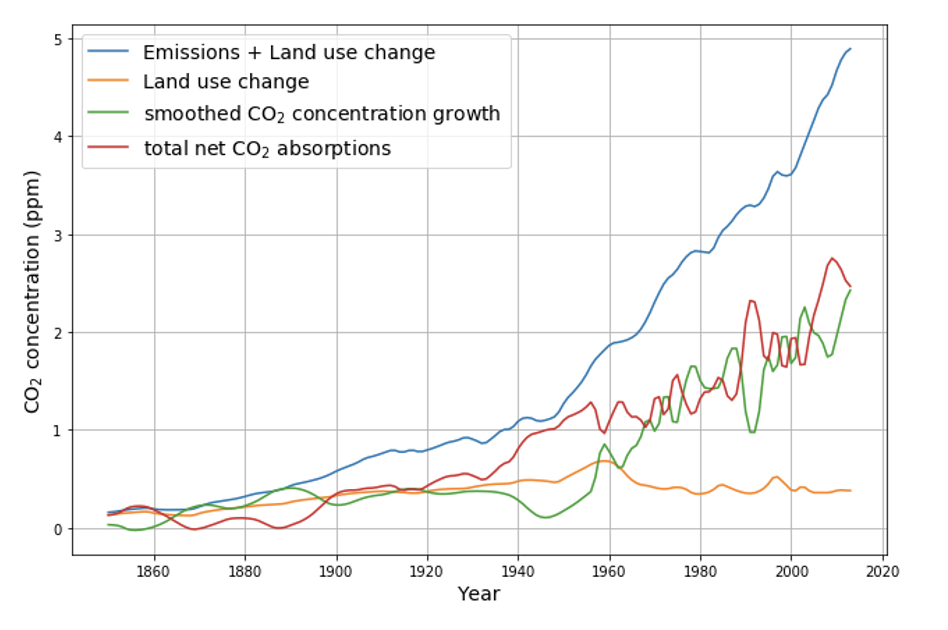
The assumption of approximate linearity of the relevant absorption processess is visualized with a scatter plot, relating the effective CO2 absorption to the CO2 concentration.

We see a long term linear dependence of the effective absorption on the atmospheric CO2 concentration with significant short term deviations, where the effective zero-absorption line is crossed at appr. 280 ppm. This is considered to be the pre-industrial equilibrium CO2 concentration where natural yearly emissions are balanced by the yearly absorptions. The average yearly absorption is appr. 2% of the CO2 concentration exceeding 280 ppm. As the data before 1950 are subject to large uncertainty, the following calculations were done based on data after 1950, resulting in a slightly smaller absorption percentage of 1.6%.
CO2 concentration as a temperature proxy
When we make predictions with hypothetical future CO2 emissions, we do not know the future temperatures. Without diving into the problematic discussion about the degree, how strong the influence of CO2 concentration is on temperature , we assume the “worst case” of full predictability of temperature effects by CO2 concentration.
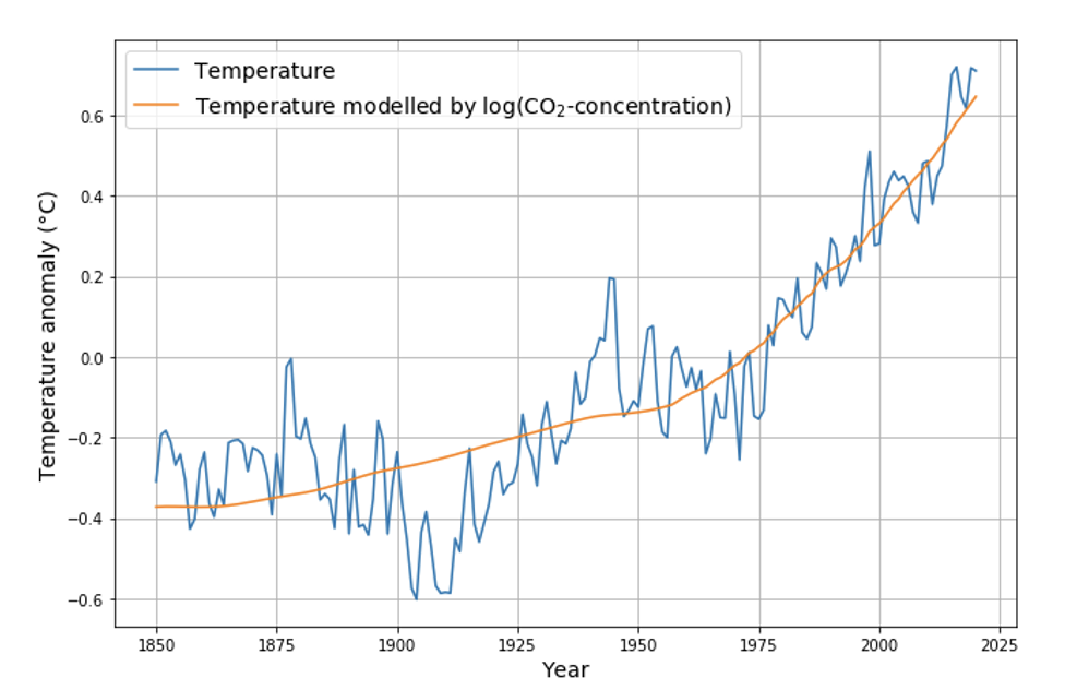
Without making any assumptions about C->T causality, the estimated functional dependence of the temperature proxy from the regression on CO2 concentration C was found to be:
Tproxy = -16.0 + 2.77*log(C) = 2.77* log(C/(235ppm))
This corresponds to a sensitivity of 1.92° C.
Model validation
The model with the assumption of constant absorption parameter and constant natural emissions is validated with a prediction of the CO2 concentration 2000-2020 based on emission data 1950-2020 and Concentration data 1950-2000.

This is an excellent prediction of concentrations on the basis of emissions and the above model assumptions. There are only small apparently variations between the predictions and the actual data. Although the model allows for varying absorptions over time, the data of the last 70 years, which is the period of the bulk anthropogenic CO2 emissions, leads to the conclusion that the CO2 absorption parameter has no significant temperature or other time-dependent component, and a current CO2 emission pulse is absorbed with a 42 year half-life time.
Future Emission Scenario
The most likely future emission scenario is the IEA stated policies emission scenario of approximately constant, slightly decreasing global emissions. The actually used data set for a realistic future projection is created by trend extrapolating the stated policies beyond 2050 and assuming that the land use change
data will follow the current trend and decrease to 0 by the year 2100 . Emissions will not be reduced to zero in the year 2100, but will remain close to the 2005 level.

Prediction of Future CO2 Concentration
From this realistic emission scenario the future CO2 concentration is recursively predicted with our model.
With the IEA stated policies scenario, i.e., no special CO2 reduction policies, a CO2 concentration equilibrium of approx. 475 ppm will be reached during the second half of this century. Based on the empirical CO2 temperature proxy equation above, this increase of CO2 concentration from 410 ppm (in 2020) to 475 ppm corresponds to a temperature increase of 0.4 _C from 2020, or 1.4°C from 1850.
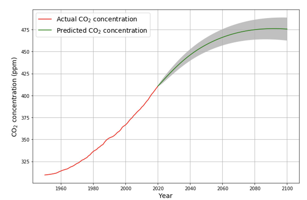
Concluding, we can expect a maximum CO2 concentration level of approximately 475 ppm in the second half of this century. At this point, the emissions will be fully balanced by the absorptions, which is by definition the “net zero” situation.
Assuming the unlikely worst case that CO2 concentration is fully responsible for all global temperature changes, the maximum expected rise of global temperature caused by the expected CO2 concentration rise is 0.4 _C from now or 1.4°C from the beginning of industrialisation.
Therefore, if we keep living our lives with the current CO2 emissions – and a 3%/decade efficiency improvement, then the Paris climate goals are fulfilled.

“given the anthropogenic emissions and the limited capability of oceans and biosphere to absorb the surplus CO2 concentration. This has led to conclusions of the kind that a certain increasing part of anthropogenic emissions will remain in the atmosphere forever.”
There’s no reason to think the biosphere limit, if it can be reached, will be reached before we reach our limit to CO2 production from limited fossil fuels.
“we can expect a maximum CO2 concentration level of approximately 475 ppm in the second half of this century.”
I did a similar analysis for my book and came out with a similar figure, 500 ppm for 2075 and then slow decline.
Pingback: Emissions and CO2 Concentration: An Evidence Based Approach - Climate- Science.press
‘…if we keep living our lives with the current CO2 emissions – and a 3%/decade efficiency improvement, then the Paris climate goals are fulfilled.’
Good news – everyone is happy!!!
Not everyone is happy. Those whose living and reputations are dependent on us living under the Sword of Damocles will not be happy.
You’d think people would be happy to hear that PM2.5 doesn’t kill anyone and that humanity didn’t cause the ozone hole but no – Western academia continues to blame modernity for every imagined ill there is well at the same time fight like Greeks to maintain the highest standard of living they can, mostly at the expense of those who are far more productive to the wealth and health of society.
“The most likely future emission scenario is the IEA stated policies emission scenario of approximately constant, slightly decreasing global emissions.”
Why isn’t this used by the IPCC if it is accepted as the most likely? Why believe the UN?
If a man’s paycheck is dependent upon …….
Never believe any bureaucracy’s statement. Been there, done that, got the scars. Its all politics.
Regarding IPCC, there is a saying in Germany (I live in a wine growing area): “Each barrel smells after its first casting”. When the IPCC was founded, the world was still under the impression of a 30 year exponential growth (4%) of carbon emissions. In Germany we called it “economic miracle”. Although the relative emission growth began to decline in 1970 (first peak oil in USA, 3 years before the oil crisis), most climate scientists were convinced that this growth would continue “forever”, so much, that some of them build the exponential emission growth into their model (see e.g. Oeschger & Siegenthaler in my paper). In the same spirit of continued exponential growth RCP8.5 was defined.
Although today most scientists are aware that RCP8.5 ist completely unrealistic (there is not enough fossile carbon to sustain that scenario for more than a few decades), it is kept with the argument of model comparabililtiy. Politically this is fatal, because it encourages dooms day alarmists.
IPCC has several scenarios – the one that comes closest to the stated policies scenario of the International Energy Agency (IEA), is RCP2.6.
Those who follow Roger Pielke jr. will recognise that there is as slow, much too slow, shift towards less alarmistic scenarios.
IEA is an organisation far from “climate denial”, on the contrary, they are pushing strongly decarbonisation. “Stated policies” is their “worst case” scenario. It reflects the current active government policies – this obviously already includes a certain amount of carbon reduction in numerous countries. It is therefore not a complete “laisser faire” scenario.
Those who reject stated policies as the most likely scenario, may please come forward with valid arguments. But note, it is not my scenario, but IEA’s.
You can’t look at natural CO2 absorption without looking hard at the oceans. Around 85-90% of the dissolved CO2 is actually in the thermally unstable alkaline earth bicarbonate form. The concentrations of the alkaline earth ions (Mg2+ and Ca2+) are about 8x higher than the bicarbonate ions. In cold water, the alkaline earth bicarbonates will stay dissolved. However, in warm water, with the help of shell forming microscopic animals it decomposes to alkaline earth carbonates which precipitates out and CO2 which might be emitted as a gas or re-dissolve.
Since the precipitation process requires warm shallow seas, warming seas should accelerate this process. We’ve seen many stories of coral atolls growing rather than disappearing under the waves. Could that be evidence of this process occurring more quickly in a warming world?
You may want to read the full paper, where we explained that this is a complementary approach, which makes use of the well accepted carbon budget equation, where actual absorptions are not determined by analysing the individual mechanisms but from the measured emissions and concentration changes. In order to build the model we only need to assume that the individual absorptions are a linear function of concentration. This has been proven by Ari Halparin, whom I refer to in the paper.
Well,
Maybe I should mention an older story.
In the late 90s, 5 multi National companies, And a few Nations, spend a “billion dollar ” or so on a refined climate modell.
The public super computer that ran climate model where not that Great, so some larger private sector systems where used.
This work, was later mentioned by Guvenor Arnold Schwarzenegger, when he wanted a model Just for California,
And he got one, i think.
Back to the private sponsored model.
It showed, that with current CO2 emissions, we would get a future close to what RCP 2.6 showed.
And, there was a smal propabillity that the next 20- 30 years will see some colder years.
If i remember correct, minus 0,2-0.4 on global average.
The model ran unril 2060. Not a 100 years.
The uncertanty rise a lot more than 60 years ahead.
This is from mye memory, so plz, forgive if i do not remember it all a 100%.
It was shown in a closed session at a large Company around 20 years ago. So far, it matches reality pretty good.
Why not make it public ?
Who knows, something about an economic advantage…
But i asked, how long will it be secret ?
2020, did they say, so for a climate scientist, this modell should be something you could study today.
It might be outdated, but it was pretty good.
Later, Japan build the first dedicated super computer, for climate modell. Was an IBM system.
I whatch the climate subject a little, And of what i can see.
The polar regions are gjetting colder.
If this continue, And it is a big IF.
Then we would enter a colder period, which will be something.
( And most likely debated )
We will see, in a few years from now.
Now that’s interesting and a complete crock!
The oceans are currently absorbing CO2. The solubility of CO2 in water decreases with temperature. There will be a point where the oceans will start to expel CO2 into the atmosphere. Also, as the earth warms, ocean circulation slows down and CO2 will saturate at the water’s surface. I suspect this “paper” doesn’t account for any of that.
This is why this stuff is never taken seriously by the scientific community. It has nothing to do with suppressing the “truth.”
My Bad – I forgot to read Al Gore’s book
Do you mean rock (as in sedimentary rock) rather than crock?
How you ever heard of limestone?? Do you know it from alkaline earth precipates in warm shallow seas? If you look at the vertical faces of the mile deep Grand Canyon, that is limestone and it represents about 40% of the depth of the canyon that’s been cut out by the Colorado river. Those rock formations extend hundreds of miles. Have you heard of the Dolomites in Italy? These are carbonate rocks originally formed in warm shallow seas that are now mountain ranges. Mother nature has been sequestering CO2 as carbonate rocks for hundreds of millions of years. Why would she stop now?
What’s your point? I’m talking about CO2 dissolved in the oceans. That is a significant sink for CO2. If that is no longer true, we are in deep trouble.
The problem with climate denial pseudo-science is that something is always left out. That why none of it is taken seriously by the scientific community. The only ones taking it seriously are those who think they understand the science.
Have a look at this reference https://rwu.pressbooks.pub/webboceanography/chapter/5-5-dissolved-gases-carbon-dioxide-ph-and-ocean-acidification/#:~:text=Most%20of%20the%20CO%202%20dissolving%20or%20produced,and%20little%20gets%20absorbed%20back%20into%20the%20air.
where it says:
“Most of the CO2 dissolving or produced in the ocean is quickly converted to bicarbonate. Bicarbonate accounts for about 92% of the CO2 dissolved in the ocean, and carbonate represents around 7%, so only about 1% remains as CO2, and little gets absorbed back into the air. The rapid conversion of CO2 into other forms prevents it from reaching equilibrium with the atmosphere, and in this way, water can hold 50-60 times as much CO2 and its derivatives as the air.”
In other words, you can’t look at CO2 dissolved in water or the oceans simply as a dissolved gas.
https://en.wikipedia.org/wiki/Carbonic_acid#:~:text=The%20hydration%20equilibrium%20constant%20at%2025%20%C2%B0C%20is,into%20carbonic%20acid%2C%20remaining%20as%20CO%202%20molecules.
That’s not true most of CO2 absorbed stays as CO2. Why do you keep carbonated beverages cold? If what you said were true, there would be no need.
It’s a question of pH. Carbonated water has a pH of 4.5 and at that pH the CO2 is mostly a dissolved gas and carbonic acid. You can see that from the first chart in thechemical equilibrium section of the reference you sent. The pH of the oceans however is around 8 and that same chart shows that the bulk of the CO2 exists as the bicarbonate with a small portion as carbonate and the smallest portion as CO2. That graph shows why CO2 most as the bicarbonate in the oceans.
You don’t need to “suspect”, if you read the actual paper. We have included a discussion, references, and ako proof that there is no indication whatsoever for a saturation
Really? NASA disagrees with you. I would say we don’t know a lot about how the oceans absorb CO2 and what the limits are. Certainly not enough to start claiming that climate change is not a problem.
https://earthobservatory.nasa.gov/features/OceanCarbon
JJ, did you bother reading what your referenced link actually said? Even its included graph show no speculated issue until oceans exceed 30℃; get real. It did show that CO2 absorption/exhalation varies naturally with ocean oscillations such as the AMO.
Its modeling is a joke: The woman doing it thinks she can model ocean CO2 concentrations from atmospheric measurements and blathers on about a whole bunch of speculative climate issues.
In no way does it counter anything presented here.
Let’s look at that paper.
It assumes that fossil fuel emissions are at a peak and will decline slightly in the future. How does that happen? If population increases and demand for energy increases, how do fossil fuel emissions slightly decline? The only way that happens is if renewables are a big part of the picture.
The second problem is that the theory is too simplistic. How do you come up with an equation with one independent variable that takes into account adsorption. It’s a glorified curve fit and I wouldn’t use it to extrapolate into the future. Climate models do the same thing, and they take into account many factors. They’re not predicting: “Don’t worry be happy.”
The third problem is that he doesn’t have a radiation model. That has a lot to do with the relationship between CO2 concentration and surface temperature.
I was going to read the original paper. Then I saw that the publisher was MDPI. Who is MDPI? It’s a Chinese outfit — open access pay-to-publish. These type organizations have shoddy peer review. It’s where you go if you know that your paper is going to be in trouble if it goes through rigorous peer review.
You don’t have to take my word for it. Here’s a summary of MDPI’s checkered past:
https://en.wikipedia.org/wiki/MDPI
You make a good case for the oceans not being saturated based upon observations and references. However the reasons for this are based on the oceans mildly basic pH which means it can hold extremely large quantities of CO2 in the bicarbonate form, it can sequester CO2 when limestone and dolomite precipitate out and the molar concentration of alkaline earth elements Mg++ and Ca++ are 8x higher than that of the bicarbonate ions.
As it gets warmer, it will absorb slightly less. This is well accounted for in their methodology. Especially since we’ve already observed more warming than we can expect. What they don’t account for is the lag in land biosphere uptake.
Biosphere uptake lags emissions/concentrations substantially. The land biosphere takes in an increasing portion of emissions every year. Soil and microbial effects lag, also epigenetic responses. Every year the biosphere takes in more. In the 90s it was about 25% of emissions, today it’s close to 30% even as emissions went up substantially. This also makes the land better at handling water.
See full 🧵 https://mobile.twitter.com/aaronshem/status/1126891477857198081
The graphs of the seasonal variations in MLO atmospheric CO2 concentration typically peak in May (only sometimes in April). It strongly suggests that there is at most a couple week lag in the response of concentration to photosynthetic activity. The problem is that vegetation doesn’t gulp it all down at once. Plants grow all Summer long, and can use more CO2 as they get bigger and produce more leaves. So, CO2 declines all Summer and comes to an end with killing frosts, reaching a low in September or October.
Clyde, you don’t happen to know of CO2 data that can be used to track night and day differences over decades do you?
Clyde, there are changes to soil and plant biology that happen over years.
I’m aware of the soil changes that happen over years, but it is not an area of my expertise. I’m sure that there are some longitudinal studies that have tracked changes.
You asked, “… CO2 data that can be used to track night and day differences over decades do you?”
I’m not sure what you are looking for. I’ve seen studies that compare daytime photosynthesis and nighttime respiration, but I don’t recollect seeing any long-term studies for a particular area.
JJ: As we have been emitting CO2, about half has been taken up by sinks on land and in the ocean. We know that only the top 50 m of the ocean is mixed during any year because changes in temperature with the seasons can only be detect to that depth. Over longer periods of time, we have measured mixing into the deep ocean by tracking CFCs that began to be produced only in the 20th century and a pulse of radioactive 14CO2 produced by atmospheric testing of atomic bombs. It is going to take a millennium or so for the extra CO2 we have released to reach most of the deep ocean. So, while people fear that the airborne fraction of CO2 released by burning fossil fuels could drop over the next century as land sinks saturate, over the following millennia the airborne fraction will decrease as more an more CO2 ends up in the deep ocean. IIRC, pre-industrially, there was 1 GtC in the atmosphere for every 64 GtC in the ocean and if ocean pH didn’t change, the CO2 released by man would eventually partition into the deep ocean with the same ratio. However, the rising pH from more CO2 means the ratio will end up somewhere near 10:1. So IIRC even if we reach 800 ppm in the atmosphere, that will drop below 400 ppm as the deep ocean takes up those emissions over the next millennia. The IPCC prefers to focus on the much longer period that will be required to “permanently” bury our emissions as CaCO3.
I’m sorry I haven’t retained this information as confidently as I would like. Some of this was discussed in a post at CE by Nic Lewis and in reference xiv (below) in that post. I hope my memory isn’t misleading you.
https://judithcurry.com/2018/12/11/climate-sensitivity-to-cumulative-carbon-emissions/#_edn16
https://agupubs.onlinelibrary.wiley.com/doi/full/10.1029/2006GB002810
Here’s the thing.
All you said is well and good, but the burning of fossil fuels and the subsequent creation of CO2 has outstripped the ability of earth’s natural processes to remove it. Until the production of CO2 from fossil fuels burning falls below the removal rate the CO2 in the atmosphere will continue to increase and the planet will continue to warm.
How high could the temperature go? Look at the planet Venus. Venus is roughly the same size and mass as the earth. It has highly reflective clouds and absorbs less solar energy than the earth. Based on its distance from the sun, its temperature should be 60 degrees C. The actual temperature of Venus is 460 degrees C. That is due to the greenhouse effect of CO2. Venus has massive amount more CO2 in its atmosphere than the earth.
Implying the Earth could get as hot as Venus by burning fossil fuels is a l — i — e.
Watch who you are calling a liar!
I implied no such thing. What I stated is scientific fact. Long before the earth has an environment similar to Venus, the human race will cease to exist. Problem solved? Maybe. It’s possible that some unknown processes are triggered that continue to increase the CO2 in earth’s atmosphere. We don’t have a good handle on the quantity of greenhouse gases that will be released by melting ice and melting permafrost. Not that it matters, because there will be no humans left to study it.
We don’t have to become Venus to end human life on this planet. Burning the known reserves of fossil fuels on this planet will be sufficient to end human life or severely contract it.
” Burning the known reserves of fossil fuels on this planet will be sufficient to end human life or severely contract it.”
Lying buffoon
JJB comment ‘ “We don’t have a good handle on the quantity of greenhouse gases that will be released by melting ice and melting permafrost.”
JJB – I thought you were the science expert –
Do we already know that from the prior periods which were much warmer?
Oh wait – the planet earth didnt go into that death spiral from all that co2 emitted from the melted perma frost – or did it ?
Perhaps you could help us with your exemplary knowledge of science history – you could even consult appleman.
Hope you notice my sarcasm – hope you would catch one of the many contradictory myths embodied with the alarmist version of science.
JJ: The processes by which CO2 is taken up into plants and soli may have some complications, but the take up of CO2 by the deep ocean is extremely simple. Wind and waves mix the top 50 or so meters of the ocean continuously, quickly producing a (pH-dependent) equilibrium distribution of CO2 (and H2CO3, HCO3- and Co3–) between the atmosphere and the ocean. Deep water forms in cold, salty locations and settles towards the bottom of the ocean, The deep water formed contains trances of CFC’s and C14 and we have tracked its progress.
As for Venus, the atmosphere is about 90% CO2 and the atmospheric pressure is about 100 times greater than on earth, meaning that there are 250,000 times as many CO2 molecules per unit volume on Venus as on Earth. Even worse, the high pressure and temperature causes the absorption band of CO2 to broaden dramatically. There is no “atmospheric window” on Venus for thermal IR to escape to space.
Venus’s atmosphere is 96% CO2. Mars atmosphere is 95% CO2. Mars has is much colder than Venus. It has nothing to do with the fact Mars is much further from the sun. It because the CO2 effect depends on absolute concentration — not relative concentration. Venus has much more CO2 than Mars.
Pressure can broaden the CO2 absorption bands. It really doesn’t matter because currently CO2 on Venus is absorbing all available energy that Venus produces in the CO2 absorption bands. CO2 can’t make Venus any hotter.
JJ wrote: Pressure can broaden the CO2 absorption bands. It really doesn’t matter because currently CO2 on Venus is absorbing all available energy that Venus produces in the CO2 absorption bands. CO2 can’t make Venus any hotter.
JJ, surface temperature and temperature at other altitudes can be controlled by upward radiative cooling or convention of heat and latent heat. The temperature profile with altitude is controlled by which of these processes dominates (moves heat the fastest). When convection dominates vertical transfer of heat, the result is a lapse rate (change with altitude) that is roughly linear with altitude. (The slope depends on the heat capacity of the atmosphere and the heat of evaporation of the moisture it contains on Earth). When radiation dominates the vertical transfer of heat (and no downward absorption of SWR, say by ozone, makes things complicated), the lapse rate is linear with pressure (the density of the absorbing gas). On Earth, the lapse rate is roughly linear with altitude from the surface to the tropopause (10-17 km depending on latitude), so we know convection is the dominant mechanism of heat transfer. The surface temperature below a tropopause at 12 km is 6.5 degC/km*12 km = 78 degC higher than the temperature at 12 km above the surface. At that altitude, all of the heat that needs to escape to space as radiation to maintain a stable temperature can escape at radiation through the thinner drier atmosphere at 12 km.
On Venus, there is 100 times as much atmosphere as on the Earth and 100 times the pressure at the surface. Probes sent to Venus have show that the lapse rate is also linear on Venus, which tells us that convection also dominates vertical heat transfer on Venus (and their is no water vapor and latent heat, which is the major form of convection on Earth). The lapse rate is 10 degC/km, as expected from the heat capacity of CO2. However, because there is so much more atmosphere, this linear lapse rate extends from the surface to roughly 50 km above the surface, making the surface roughly 500 degC warming than the top of the atmosphere where the CO2 is thin enough to allow radiative cooling to space balance incoming and outgoing radiation. This balance includes the fact that Venus has a higher albedo than the Earth and more intense SWR from the sun.
So, more CO2 on Venus can make the surface warmer by extending the distance there is a linear lapse rate from high in the atmosphere radiative cooling to space sets the temperature. So, if the atmospheric pressure was 200 atmospheres on Venus, it might be 70 km from the top of the linear lapse rate to the surface and 200 degC warmer.
The above explanation involving lapse rates and convection fells uncomfortable with our conception of warming by a greenhouse effect based on absorption of outgoing thermal IR. However, that explanation has long been oversimplified: If there were no lapse rate on the Earth and the atmosphere were isothermal, rising GHGs wouldn’t produce any GHE. Rising GHGs are not producing any radiative forcing over Antarctica, where the air descending from the tropopause is about the same average temperature as the cold surface. To have a GHE, photons need to travel far enough for there to be a significant difference in temperature between absorption and emission. There is an article on Schwarzschild Equation for Radiative Transfer in Wikipedia that might help you understand the deepest physics that produces our GHE.
I’ve read this before, and it’s based on the belief that the CO2 effect on earth’s surface radiation is saturated. That means that any impact of CO2 on temperature has to be coming from radiation absorption in the upper atmosphere. That’s not true.
The CO2 effect saturates in the lower atmosphere. That means for a fixed source of IR, CO2 can’t absorb any more IR no matter how much more CO2 is added. The problem with that is the earth is not a fixed source of IR. As the planet warms, it radiates more energy that CO2 can absorb. That energy warms the planet which generates more energy that CO2 can absorb, and so on, and so on. There is a point where that ends or slows down, but not before the human race is toast. Even if the atmosphere is isothermal the planet will continue to warm with increasing CO2 because of the effect I just described.
Here’s a spectrograph of Venus:
https://scholarsandrogues.files.wordpress.com/2011/05/venus-co2-spectrum-lg.jpg
This spectrograph is different from my other one. It shows absorbance instead of transmittance. See the three peaks with an absorbance of 1? That’s the 3 absorbance bands of CO2. They are saturated. Meaning CO2 is absorbing all available energy and additional CO2 cannot cause any more warming because there is no more energy to absorb.
The CO2 absorbance band on the right is the 15 mm band that is causing climate change on earth. The area under the blue curve is the radiant energy of Venus. Notice that there is very little energy for the band to absorb. As the temperature of the planet increases, the blue curve moves left toward shorter wavelengths. There is even less energy for this band to absorb. It can no longer impact planetary temperature no matter what the absorbance. The width of the band is because of pressure broadening.
The two absorbance bands at the peak of the radiant energy curve set the temperature of the planet. They are balanced across the peak. What does that mean? Think about. If the planet’s temperature increases the radiant energy curve is shifted to the left. There is less energy for CO2 to absorb. That means as soon as whatever energy source is causing the temperature increase is taken away, the temperature of the planet will drop to the temperature where the outer CO2 bands balance across the peak. A similar process occurs if the planet cools. The situation on Venus is at steady state with regards to CO2.
What you are talking about would have to create a new permanent energy source to drive the temperature of the planet higher. Otherwise, as soon as it dissipates, the planet will go back to the original steady-state
JJ: You must have read somewhere that the radiative forcing (the reduction in radiative cooling to space) caused by rising CO2 varies with the logarithm of the CO2 concentration. Going for 300 ppm to 600 ppm is about 3.6 W/m2 of radiation. From 600 to 1200 ppm is another 3.6 W/m2. If we dug up and burned all of the coal and other fossil fuels we believe are available on the planet, we probably won’t get above 1000 ppm. Hundreds of millions of years ago, we might have had 4000 ppm of CO2. Each doubling of CO2 if believed to result in 3 +/- 1 degC of warming according to the IPCC consensus. I doesn’t make sense to talk about the Earth turning into Venus.
If Venus has 250,000-times more CO2 in its atmosphere than the Earth does, where did all of our CO2 go. To start with, our oceans hold about 100 times as much CO2 as our atmosphere and Venus doesn’t have oceans. In the ocean, dissolved CO2 and Ca++ and Mg++ ions that have been washed into the ocean from land get together to make calcium and magnesium carbonate. There are massive deposits of both on our planet (such as the White Cliffs of Dover).
There is no doubt that rising CO2 and other GHGs slow radiative cooling to space. The law of conservation of energy demands that the planet to warm (somewhere) until balance is restored between incoming and outgoing radiation – unless something else changes too. Another LIA would help or a quieter sun. So far, nothing on the horizon is a good bet to prevent warming. The real question is how much warming there will be per doubling.
Here’s the thing.
The law of diminishing returns applies to absorption of radiation by CO2 molecules in the atmosphere. It only applies for a fixed energy source. The earth is not a fixed energy source. As temperature of the earth rises, the earth radiates more energy that CO2 can absorb. The example you gave doesn’t apply.
Current thinking is that the CO2 in the lower atmosphere absorbs all the earth’s radiation in its band and none of that radiation escapes. What you see at TOA in the CO2 band is radiation generated in the upper atmosphere. That’s where all the new absorption is occurring. The ppm of CO2 in the atmosphere doesn’t vary much with altitude, but the quantity of CO2 does. The higher you go in the atmosphere the less the number of CO2 molecules. Radiant energy generated in the lower atmosphere is absorbed by these molecules. As CO2 is added to the atmosphere more molecules wind up in the upper atmosphere to absorb more radiant energy.
It’s a lot more complicated than it seems.
Franktoo wrote:
If we dug up and burned all of the coal and other fossil fuels we believe are available on the planet, we probably won’t get above 1000 ppm. Hundreds of millions of years ago, we might have had 4000 ppm of CO2.
Where do you think that carbon (in the 4000 ppm CO2) went?
In 2012, Neil Swart and Andrew Weaver wrote a commentary:
“The Alberta oil sands and climate,” Neil C. Swart and Andrew J. Weaver, Nature Climate Change, 2012.
https://www.nature.com/articles/nclimate1421/
They calculated that the total known reserve of carbons on Earth was 125e17 g C (=12,500 GtC), enough to raise the global temperature by 18.78 (9.46–32.73) C.
I’ll let you estimate the ppm CO2 in the atmosphere for that, but it’s certainly much greater than 1000 ppm.
JJ writes: I’ve read this before [radiative forcing], and it’s based on the belief that the CO2 effect on earth’s surface radiation is saturated. That means that any impact of CO2 on temperature has to be coming from radiation absorption in the upper atmosphere. That’s not true.
No, radiative forcing is calculated from the fundamental physics of how radiation intensity is change as it pass through an atmosphere that both absorbs and emits. Most of us get taught about absorption and separately about emission of blackbody radiation. To measure absorption in the lab, we start with a light source with a glowing filament that is several thousand degK – so we can ignore the tiny amount of thermal IR emitted by the sample (and the entire lab.) However, in the atmosphere the amount of thermal IR emitted is comparable, no basic undergraduate course tells us how to deal with that. Then you are taught about blackbody radiation and may see a derivation of Planck’s law. However, that derivation starts by assuming radiation where absorption by and emission from the medium it is passing through is in equilibrium. This isn’t the general situation in our atmosphere. To learn how radiative forcing is calculated you need to learn some new physics: Schwarzschild’s equation for radiative transfer. This equation deals with the phenomena of saturation. It also simplifies to Beer’w law for absorption when emission is negligible and to Planck’s law when absorption and emission are in equilibrium.
https://en.wikipedia.org/wiki/Schwarzschild%27s_equation_for_radiative_transfer
Unfortunately, Schwarzschild’s equation is a differential equation that must be integrated over the path radiation travels (say from the surface to space for radiative forcing) and over all relevant wavelengths, so their is nothing intuitive about this physics and the output of numerical integration. However, the process of performing such calculations has been automated by programs such as Modtran:
http://climatemodels.uchicago.edu/modtran/
Then you need to understand that temperature in an atmosphere is controlled by heat transfer by both radiation and convection. In the 1960s. Manabe was the first to realize that the atmosphere was in a state of radiative-connectivity equilibrium. If all of the heat from incoming SWR can’t escape as thermal IR as fast as it arrives at the surface, the lapse rate becomes unstable and convection carries heat upward until the atmosphere it thin enought for it to escape as radiation.
The best place to learn about the physics of climate science is scienceofdoom.com.
I never mentioned “radiative forcing.” What I was pointing out is that radiation in the 15mm band leaving the earth is not from the surface of the Earth. It is generated in the atmosphere.
The second point I was trying to make — apparently badly — is that an isothermal atmosphere is not a solution to climate change because the earth is not a fixed source of radiative energy.
Pressure can broaden the CO2 absorption bands. It really doesn’t matter because currently CO2 on Venus is absorbing all available energy that Venus produces in the CO2 absorption bands. CO2 can’t make Venus any hotter.
See the sidebar on page 37 of:
Pierrehumbert RT 2011: Infrared radiation and planetary temperature. Physics Today 64, 33-38
http://geosci.uchicago.edu/~rtp1/papers/PhysTodayRT2011.pdf
“Saturation fallacies”
“The path to the present understanding of the effect of carbon dioxide on climate was not without its missteps. Notably, in 1900 Knut Ångström (son of Anders Ångström, whose name graces a unit of length widely used among spectroscopists) argued in opposition to his fellow Swedish scientist Svante Arrhenius that increasing CO2 could not affect Earth’s climate. Ångström claimed that IR absorption by CO2 was saturated in the sense that, for those wavelengths CO2 could absorb at all, the CO2 already present in Earth’s atmosphere was absorbing essentially all of the IR. With regard to Earthlike atmospheres, Ångström was doubly wrong. First, modern spectroscopy shows that CO2 is nowhere near being saturated. Ångström’s laboratory experiments were simply too inaccurate to show the additional absorption in the wings of the 667-cm−1 CO2 feature that follows upon increasing CO2. But even if CO2 were saturated in Ångström’s sense—as indeed it is on Venus—his argument would nonetheless be fallacious. The Venusian atmosphere as a whole may be saturated with regard to IR absorption, but the radiation only escapes from the thin upper portions of the atmosphere that are not saturated. Hot as Venus is, it would become still hotter if one added CO2 to its atmosphere.”
Pierrehumbert RT 2011: Infrared radiation and planetary temperature. Physics Today 64, 33-38
I’m aware of the argument that the CO2 effect is not saturated. I agree with the point that spectroscopy shows that it isn’t. I don’t agree with the idea that CO2 radiation that emitted in the upper atmosphere can be absorbed, and the Venus can continue warming.
My first counter argument is that when does that stop. In theory you could make the planet Venus hotter than the sun and violate the second law of thermodynamics.
Here’s something that explains why the temperature of the planet won’t increase no matter how much CO2 is added to the atmosphere of Venus.
https://scholarsandrogues.files.wordpress.com/2011/05/venus-co2-spectrum-lg.jpg
That is an IR spectrograph of Venus. The 3 CO2 absorption are the ones that are absorbing 100% of the IR radiation available to them.
What happens when the temperature of Venus increases? The planet emits more radiant energy at every wavelength and the energy distribution shifts to shorter wavelengths. That means on the spectrograph Venus’s radiant energy profile shifts left and is higher. CO2 absorption bands to the left of the peak have more energy to absorb because of the shift. Absorption bands to the right have less energy to absorb because of the shift.
Once an absorption band is on the right side of the peak, it can no longer cause the planet to warm That’s because with each temperature increase less energy is available for the band to absorb. That means the amount of energy that the earth absorbs from the absorption band is less — cooling the planet.
Look at the three CO2 absorption bands. Two are to the right of the peak and one is to the left. They are in balance. If the temperature of Venus increases, Venus radiates less energy that the CO2 absorption bands can absorb. That means CO2 absorbs less radiation. The effect is to cool the planet. If the temperature of Venus decreases more energy is available for CO2 to absorb. The effect is to warm the planet. Another source can warm the planet higher than CO2 but not additional CO2.
Thank you for the though provoking article.
This wasn’t the only article I read today from MDPI, since reading Peter Stallinga’s Dec 2022 paper earlier today “Residence Time vs. Adjustment Time of Carbon Dioxide in the Atmosphere“, I at least found there are more contrasting opinions to weigh.
Excerpt from the Dengler-Reid paper abstract:
“Observations lead to the model assumption that carbon sinks, similar to oceans or the biosphere, are linearly dependent on CO2 concentration on a decadal scale. In particular, this implies the falsifiable hypothesis that oceanic and biological CO2 buffers have not significantly changed in the past 70 years and are not saturated in the foreseeable future.”
Excerpt from the Dengler-Reid conclusion:
The assumption that CO2 concentration can be used as an upper limit proxy for temperature, i.e., a part of the temperature changes that can be explained by CO2 concentration.
The Dengler-Reid paper assumes a pre-industrial equilibrium and the increase in CO2 is due solely to man-made emissions.
The Stallinga abstract:
We study the concepts of residence time vs. adjustment time time for carbon dioxide in the atmosphere. The system is analyzed with a two-box first-order model. Using this model, we reach three important conclusions: (1) The adjustment time is never larger than the residence time and can, thus, not be longer than about 5 years. (2) The idea of the atmosphere being stable at 280 ppm in pre-industrial times is untenable. (3) Nearly 90% of all anthropogenic carbon dioxide has already been removed from the atmosphere.
Excerpt from Stallinga’s paper:
However, we expect the most likely improvement to the model to come from abandoning the idea that the residence times τa and τs are constant. They, in fact, are very much dependent on temperature. As an example, the ratio between the two that tells us the concentrations (and, thus, the masses) between carbon dioxide in the atmosphere and in the sink, if we assume this sink to be the oceans, is governed by Henry’s Law, and this concentration ratio is then dependent on temperature. When including such effects, we might even conclude that the entire concentration of carbon dioxide in the atmosphere is fully governed by such environmental parameters and fully independent of human injections into the system.
CO2 significantly lags SST, which supports Peter Stallinga.
https://i.postimg.cc/qRDB86H9/12m-ML-CO2-lags-12m-SST-by-5-months.png
It would be nice to see an open discussion between the authors of these two papers together with Dr. Curry on a podcast/video moderated by her, to air these important differences in opinion.
If there is interest, I am ready for a live discussion.
For now, I’d like to refer to reference [11] in our paper, where Gavin Cawley nicely explains the important difference between residence time and adjustment time – they are by no mean identical.
In our paper we point out, that all those emissions and absorptions that are neutralising each within the given time interval, cannot be visible in the final balance. It is as with a bank account: You may have many deposits (=100 natural and 1 human emissions) of 101 $ in total and many payments (=absorptions) of 100 $ in total. Your final visible balance sheet shows you only 1 $. The 100 $ determine the residence time whereas the 1 $ determines the adjustment time.
JJB – Henry”s law WILL have an effect on the bicarbonate equilibrium. CO2 + H2O is the first reaction in the equation. You claim to be a chemical engineer? Maybe you got a little rusty.
I’m not rusty at all. I’ve done a similar system. You have to build a quasi-equilibrium model, or handle it as an electrolyte problem.
“Henry”s law WILL have an effect on the bicarbonate equilibrium. CO2 + H2O is the first reaction in the equation.”
What does that mean? Henry’s law is inappropriate for this system. It is for the VLE of an insoluble, inert gas. Think oxygen or nitrogen in water.
Why don’t you stick with what you’re good at. BTW, what are you good at?
NIST seems to disagree with your take on Henry’s law and CO2. Maybe you need some ChemE adult education courses.
https://webbook.nist.gov/cgi/cbook.cgi?ID=C124389&Mask=10
Try again!
https://chemistry.stackexchange.com/questions/66168/is-henrys-law-sufficient-for-calculating-co2-solubility
Wrong question. But nice try.
Bob, thanks for linking to Stallinga 2023. I was aware of his 2020 paper, but had not seen this one. His analysis and findings are consistent with others challenging the IPCC paradigm for CO2. My synopsis with exhibits is here:
https://rclutz.com/2023/03/26/co2-fluxes-not-what-ipcc-telling-you/
I read the introduction to the underlying paper and my opinion is that it’s complete BS. If you can’t dazzle with brilliance, baffle them with BS.
It talks about sinks and removal rates but misses the obvious. The greenhouse effect of CO2 depends on the absolute concentration of CO2 in the atmosphere. We use the relative concentration term — ppm — as a proxy. The relevant equation is Accumulation = In – Out. As long as we keep putting more CO2 in the atmosphere than is being taken out, the CO2 ppm keeps rising and so does CO2’s greenhouse effect. Since WWII we’ve been dumping CO2 in the atmosphere by using fossil fuels at ever increasing rates. The CO2 ppm in the atmosphere has been increasing in lockstep. To claim that using fossil fuels isn’t the cause of increasing CO2 ppm in the atmosphere is ridiculous. Even the fossil fuel industry won’t buy in to that nonsense.
The paper claims that CO2 in the atmosphere behaves like H2O. Another ridiculous conclusion. H2O condenses in the atmosphere. That’s why the effect is temperature limited. CO2 does not condense in the atmosphere. In fact, by raising atmospheric temperature, CO2 increases the greenhouse effect of H2O.
This is the reason you need to be leery of any paper published in a “pay-to-publish” journal. These journals have shoddy peer review. The reason authors publish in these journals is because they know that their papers could never withstand rigorous peer review.
“The paper claims that CO2 in the atmosphere behaves like H2O. ” False, the paper quotes IPCC saying atmospheric H2O is temperature dependent. It refers to Henry’s Law saying that CO2 dissolved in the ocean is temperature dependent. And it shows how warming since the end of the LIA produced outgassing of natural CO2, which didn’t stop when humans began using fossil fuels. Sorry that you are locked into a wrong paradigm.
For some reason I can’t copy the relevant paragraph, but the H2O discussion is in Section 1 Introduction’ Here he implies that CO2 behaves like water and that the CO2 concentration in the atmosphere is dependent on temperature. It isn’t.
I assume he is relying on the decrease in solubility of CO2 in water with temperature. That could be a problem in the future, but isn’t a problem right now. Seawater is currently removing CO2 from the atmosphere — not expelling it to the atmosphere. In other words what’s causing the rise in atmospheric CO2 ppm is the increased usage of fossil fuels.
Henry’s law is for non-soluble chemically inert gas. CO2 is anything but that. In the ocean CO2 reacts both chemically and biologically. Henry’s law is an inappropriate way to model its VLE.
How can the oceans on net be absorbing CO2 and be responsible for the increasing CO2 in the atmosphere? That’s why this theory is going nowhere in the scientific community. It doesn’t pass the laugh test
Lots of suppositions and circular thinking. I leave you to it.
“How can the oceans on net be absorbing CO2 and be responsible for the increasing CO2 in the atmosphere? That’s why this theory is going nowhere in the scientific community. It doesn’t pass the laugh test”
imo, the science community view doesn’t pass the smell test.
If you understood Henry’s Law properly in terms of temperature dependence under relatively constant pressure, you would know you’ve mischaracterized it, so the laugh is on you.
The growing warm area SST ≥25.6°C acts like a check valve to atmospheric CO2, so the warming of the ocean has lead to less sinking, not more, and has lead to more outgassing from the now warmer area that grew by about 50% since 1854. Both factors as well as the man-made contribution have lead to the increase of atmospheric CO2.
https://i.postimg.cc/5y9wzKdG/Latitudinal-SST-and-CO2-Solubility.png
If the ocean had not warmed since 1854, there would’ve been more sinking, less outgassing, leading to lower atmCO2 levels.
All of the rise in ML CO2 can be modeled by the temperature and size of the warm area ≥25.6°C together:
https://i.postimg.cc/gkGnpM1g/CO2-Outgassing-Model.png
Let me say it again. Henry’s Law is not appropriate for a system involving reaction and ionization. The right way to do it is with an electrolyte model. This system is so common any of the process simulators that support electrolytes should be able to handle it.
I don’t understand your obsession with CO2 in the oceans. You and others are trying to minimize the impact of burning fossil fuels on CO2 in the atmosphere. The ocean is not a source of CO2 in the atmosphere. It’s a sink and removes CO2 from the atmosphere. All you have to know is that if we stop using fossil fuels the amount of CO2 in the atmosphere will start decreasing. CO2 in the oceans can’t drive the amount of CO2 in the atmosphere higher.
Here’s an IR spectrograph of earth’s radiant energy:
https://th.bing.com/th/id/R.d75b0d49b696ecedec244862e1d2ac47?rik=MgOi1dZjld6Beg&pid=ImgRaw&r=0
The pink area under the CO2 label is the amount of the earth’s radiant CO2 is preventing from going to outer space. That energy didn’t disappear. It is warming the earth. The only conclusions one can draw is that increasing CO2 in the atmosphere is warming the earth. Burning fossil fuels is increasing the CO2 in the atmosphere.
CO2 significantly lags SST, which supports Peter Stallinga.
Anthropogenic CO2’s warming effect is immediate, therefore anthropogenic warming lags it.
But if it’s an ocean temperature problem, thermal mass means everything is going to happen very very slowly, so I can probably put off buying an EV until Monday.
As a matter of fact, we tested the hypothesis, that the global absorption coefficient might depend on the historical ocean surface temperature (HadSST). We had to reject this hypothesis because of statistical insignificance.
So you might as well wait until tuesday before buying an EV
Very interesting. Thank you.
Joachim,
You state, “the data of the last 70 years, …, leads to the conclusion that the CO2 absorption parameter has no significant temperature or other time-dependent component, …”
It is well-known that the (bi)carbonate solution rate and saturation threshold is temperature dependent. Empirical evidence shows that the rate of seasonal increase, peak, and net annual increase is related to temperature. See particularly, Fig. 3 here: https://wattsupwiththat.com/2021/06/11/contribution-of-anthropogenic-co2-emissions-to-changes-in-atmospheric-concentrations/
Also, see Fig. 5 for what happened to the range of the seasonal ramp-up phase during the 1998 and 2016 El Ninos.
How do you reconcile your quoted statement with the obvious transient behavior of atmospheric CO2 during El Nino events?
As a matter of fact, in the paper we make it clear, that obviously there is in principle a temperature dependence – the paleo data and physics prove that. And we also quote explicitely Roy Spencer, who has shown the effect of El Nino, and we discuss this.
But the question is not, if there is a temperature dependence in principle, rather we need to check if there is a temperature dependence during the time period of measurement resp. prediction.
Having said that, we take the 70 year period of high quality measurements (strictly speaking Maona Loa data only begin in 1959) and test statistically if for the full interval a temperature dependent trend can be identified. We can safely assume that periodic effects such as El Nino will average out over a long period. You can check the statistical tests we made. The error probability of the temperature (HadSST) dependent parameter is 54%. I suppose you agree that I have to come to the conclusion that the parameter is not significantly different from 0 under this condition.
Obviously there is an uncertainty regarding the future. But if there is no overall trend during the last 70 years, the best prediction for the immediate(!) future is to assume the same. Until 2080 we speak of less than 60 years, which is less thank our investigated time interval.
Additionally we made an ex-post prognosis for 2000-2020 based on data from 1950-1999 – the result is of incredible quality.
Compare this to e.g. Oeschger’s prognosis who predicted 590 ppm CO2 concentration for 2020.
Joachim, I didn’t understand this part:
Tproxy = -16.0 + 2.77*log(C) = 2.77* log(C/(235ppm))
Suppose for example that C is 400 ppmv. I assume “log” is the natural log, base e:
> -16+2.77*log(400)
[1] 0.5963568
> 2.77*log(400/235)
[1] 1.473305
What am I missing here?
Also, what is the origin of the 235 ppmv?
Thanks,
w.
Thanks for pointing to this – unfortunately this is a “typo”. It should be 325 ppm (more precise 322.5) , corresponding to the CO2 concentration at the time when temperature anomaly is 0, i.e. exp(16.0/2.77).
Sorry for the confusion.
Joachim, that clears up the math error, thanks much.
But I still don’t understand the logic. For example, it’s true that:
-16.0 + 2.77*log(C) = 2.77* log(C / (322.5ppm))
But it’s also true that:
-10.0 + 1.73 log(C) = 1.73 * log (C / (322.5ppm))
It’s not clear to me what you mean when you say “when the temperature anomaly is 0”, where you got the -16°C, or how you know what the atmospheric CO2 concentration was at that point in time.
I hope very much that you don’t think that -16°C is the temperature of a blackbody earth. See the post “Earth’s baseline black-body model – “a damn hard problem” for the reason why.
https://wattsupwiththat.com/2012/01/12/earths-baseline-black-body-model-a-damn-hard-problem/
w.
Unfortunately this is a type, it should be 325 ppm (to be precise 322.5), i.e. exp(16.0/2.77).
Sorry for the confusion.
Willis, as there is no reply possibility on your last post/question, I answer here. There is nothing mysterious about that equation you asked about. It is just a linear regression ( y = a + b*x) of the HadSST temperature time series as the dependent variable y and the log(CO2 Concentration) as the independent variable x. The result of an ordinary least squares method (e.g. Python OLS) is a = -16 and b = 2.77.
Beware, the HadSST “temperatures” are not actual temperatures, but anomalies.
In trying to make this more intuitive, in this blog (not in the paper) I decided to rewrite this with a single log function of a concentration ratio – obviously it didn’t become more intuitive but apparently confusing…
Thanks, Joachim, much appreciated. I’d just never seen it in that format before.
My best to you,
w.
Does anybody use CO2 data from OCO-2?
We see a long term linear dependence of the effective absorption on the atmospheric CO2 concentration with significant short term deviations, where the effective zero-absorption line is crossed at appr. 280 ppm.
I think this is where you go seriously wrong.
CO2 absorption is determined by physics, not curve fitting.
It’s far from clear that your graph exhibits a linear dependence.
We already know that parts of the Amazon are saturated and no longer a sink of CO2.
We don’t know how the future absorption rate of the ocean, as it absorbs more and more CO2. Will it stay at the same rate? Start to saturate?
You also don’t take into account feedbacks to climate change itself — the ice albedo effect, water vapor feedback, and the lapse rate feedback. These are very significant, and their effects can’t be determined by a numerical fit to a CO2 graph.
The required model depends on real physics, not linear interpolations. So your conclusions for climate sensitivity and warming at 2100 are not scientifically meaningful.
I don’t think a legitimate journal would have published your paper.
The so-called Ice Albedo Effect is overstated.
https://wattsupwiththat.com/2016/09/12/why-albedo-is-the-wrong-measure-of-reflectivity-for-modeling-climate/
“””CO2 absorption is determined by physics,
[..]parts of the Amazon are saturated and no longer a sink of CO2
[..]don’t know how the future absorption rate of the ocean”””
The processes you describe here are mainly biological.
The physical part of CO2 absorption into the oceans well enough understood (beside getting warmer for near future we are getting further away from the equilibrium concentration and thus the absorption should linearly increase).
Large scale tree cutting (not only in Brazil, the US is a leading pallet producer) is a crime, no question!
But so far the world still is getting greener, being it a Florida sized algae bloom.
This makes a linear absorption argument somewhat defendable.
morfu03 wrote:
The processes you describe here are mainly biological.
Biological absorption isn’t important?
The physical part of CO2 absorption into the oceans well enough understood (beside getting warmer for near future we are getting further away from the equilibrium concentration and thus the absorption should linearly increase).
Why linearly?
But so far the world still is getting greener, being it a Florida sized algae bloom.
This makes a linear absorption argument somewhat defendable.
Why does the world “getting greener” mean the absorption coefficient linear? Instead of a polynomial of order two, or even 3/2? What physics/chemistry/biology gives the order of the coefficient?
Biosphere uptake lags emissions/concentrations substantially. The land biosphere takes in an increasing portion of emissions every year. Soil and microbial effects lag, also epigenetic responses lag. Every year the biosphere takes in more. In the 90s it was about 25% of emissions, today it’s close to 30% even as emissions went up substantially. This also makes the land better at handling water.
See full 🧵 https://mobile.twitter.com/aaronshem/status/1126891477857198081
Areas that may have reached “nutrient limits” are small and probably have more to do with el Nino heat and drying.
The local DA: “We don’t know how the future absorption rate of the ocean, as it absorbs more and more CO2. Will it stay at the same rate?”
You won’t like more oceanic CO2, but will phytoplankton like more CO2? What happens when life is fed, DA? I suggest you go on a diet and reduce yourself.
Jungletrunks wrote:
You won’t like more oceanic CO2, but will phytoplankton like more CO2? What happens when life is fed, DA?
There are more than one variables at play.
How do phytoplankton respond to higher temperatures and higher acidification?
Your comments make it clear to me that you haven’t even looked into the actual article, where we declared the diagram that you complain about, explicitly as a “first exploratory analysis”.
Consequently you also completely missed the full analysis, which includes the fact, that the full time range from 1850-2020 would imply a temperature dependent term, and the discussion why it is reasonable to do the prediction with the more reliable measurements after 1950. Only then we are forced to the conclusion, that — also for me unexpectedly — there appears to be no more temperature dependence of the absorption coefficient.
You then also missed the extensive discussion about the linear dependence of the different absorption mechanisms, which includes the reference [7], where the physics details of the absorption mechanism are derived and shown to be linearly dependent on concentration — between possible activation offset and saturation.
You also missed the discussion in the paper, that absorption processes are a priori temperature dependent, and that all statistical tests included the temperature dependence. Only after the proof of statistical insignificance I was forced to discard temperature dependence (in the limited time range of the last 70 years).
By not reading the paper you also failed to notice the reference to a recent publication in Nature (reference [15]), providing evidence that “most ocean model underestimate uptake”.
You also missed our discussion and evaluation of a possible saturation of the oceans in the near future.
By not reading the article you are also not aware, that by sweepingly dismissing our approach, you foolishly dismiss the Bern Model of the Nobel Price winner Hasselmann, which we have shown to be mathematically equivalent to the time dependent variant of our model.
If you want to be taken serious, I recommend to be more thorough in your analysis and less arrogant in your judgement.
If you really think you have something here, you need to submit this paper to a mainstream journal that does rigorous peer review — not one of these “pay-to publish” journals, with a spotty reputation.
In your paper you make the assumption that CO2 emissions have peaked and will gradually decrease during the rest of this century. I have seen projections that claim energy consumption will increase 4xs by 2100. The only way your assumption is valid is if the efficiency of the ICE is drastically increased — not likely. The price of fossil fuels get so high that it stifles demand and kneecaps the economy — not politically acceptable. Renewables and/or nuclear become a huge component of energy generation — most likely. If option 3 is what happens, then your analysis is not much different than the IPCC’s recommendation except that the IPCC wants net zero emissions.
I am surprised by the relatively stable inpact of the land use change component indicated in the graphs since the 1960s. Urbanisation, tropical forest clearance, and agricultural changes have taken place at a global scale with consequences for CO2 concentration.
To be honest, the land use change is a puzzling element in the game. You need to be aware, that the larger you assume the LUC to be, the more absorptions you have to assume.
The Global budget (or mass conservation) constraint is very strict and unforgiving.
When publishing the paper, it was clear for me, that I have to take into account the accepted wisdom about LUC. The doubts came, when it became impossible to reconstruct the widely accepted pre-industrial concentration of 280 ppm with the proposed LUC. Therefore I had to reduce the LUC within the (very large) error bounds. Taking the reliable concentration data after 1959 the problem becomes worse w.r.t. LUC – in the paper I sticked to the given LUC data. The price was a far too low value for the natural equlibrium concentration. This I consider to be the weakest member in the chain of arguments in our paper.
But when I do a radical and unorthodox step, and drop the LUC completely for data after 1950, not only the statistical error is reduced, but I get a natural equlibrium concentration of 281 ppm (!), which is absolutely remarkable.
Things are different in the first half of the 20th century. A LUC term appears to be required, although not as large as the common wisdom suggests.
How to interpret this absolutely strange result? Have we overestimated the effects of urbanisation etc.? Is the the carbon fertilisation (over-) compensating all other adverse effects of civilisation?
These are honest open questions for me. But the numbers are as they are. I can’t find an error in them. I wish, others would recalculate these equations. It’s not so difficult….
It’s mostly a fudge factor,
It allows for the claim that the airborne fraction isn’t decreasing.
“How to interpret this absolutely strange result? Have we overestimated the effects of urbanisation etc.? Is the the carbon fertilisation (over-) compensating all other adverse effects of civilisation?”
I can’t answer the science behind any of your questions other than offer an interesting stat as it relates to your inference of “we”— all human kind: if every human on the planet (7 billion) stood shoulder-to-shoulder, they would only fill the landmass of LA; according to National Geographic. Obviously “we can” greatly influence the habitability of the planet; but you couch the important fundamental question pertaining to CO2:
are we…”(over-) compensating all other adverse effects of civilisation”.
Anecdotally, as a non scientist, I would place nuclear war at the top of the list of humans not over compensating for risk, and CO2 at the top of the list (far beyond nukes) for over compensation of risk. Both represent massive political and economic risks, both are manufactured, only one is real based on each examples relative scale of risk. Both nukes and CO2 are used for emotive political leverage, for use in the assessment and branding of risk, including: threat, fear, cost (both financial and biological). Each risk calls for collective change, only one calls for collectivist mitigation to finally eliminate all risk. The collectivist angle implicitly promises that global political hegemony is the salvation for all human kind—a utopian political destination where finally all these risks can be put to rest. The irony is that there’s no example where collectivism has solved, or resolved anything other than representing explicit dystopia. Dystopia is the real risk.
https://www.mdpi.com/1099-4300/25/2/384
This is a revolutionary paper. It undermines almost all of the IPCC assumptions on atmospheric CO2 history, stability and time parameters of residence. It supports anomalous and contradictory CO2 data that has been discarded as erroneous.
It seems straightforward. I’d love to see it challenged.
This is in fact a wild claim: “We do not have to discuss each absorption mechanism from the atmosphere into oceans or plants. From the known global concentration changes and the known global emissions, we have a good estimate of the sum of actual yearly absorptions.”
Known global emissions? How much did the boreal forest of Canada emit last year? How about the Gulf of Mexico? The Amazon? Kansas?
Nothing is measured so we have no idea. It is all fantasy. Unfounded guesses claiming to be science.
Most of the emissions probably never make it out of the local biospheres (terrestrial and oceanic) before they are absorbed nearby. We have no idea what the global emissions are nor how they change over time.
David Wojick wrote:
Known global emissions? How much did the boreal forest of Canada emit last year? How about the Gulf of Mexico? The Amazon? Kansas?
These numbers come from models, which *do* come from measurements.
David Wojick wrote:
Most of the emissions probably never make it out of the local biospheres (terrestrial and oceanic) before they are absorbed nearby.
What science says that?
Please cite it.
From the whole context of the article and the underlying paper it should be clear, that with the “known global emissions” we obviously speak only of the anthropogenic emissions. These are indeed well known are regularly published by e.g. the IEA.
If you had looked into the actual paper instead of making your premature judgement on the basis of a single sentence in the non-technical summary, you might have come to this conclusion yourself.
I agree that we don’t know the details about all natural emissions.
We don’t need to know them for making sound evaluations.
They appear in our model as the constant equilibrium concentration and the residual error. If you had looked into the paper, you would have seen that we discussed the hypothesis of the global equilibrium between natural emissions and absorptions in section 2.4.
From our ex-post prediction of 2000-2020 you can see that the residual error is remarkably small.
If you look more closely, you will notice that our prediction of the remaining concentration not only is close to the center of the error bound, but also slightly above the actual concentration.
This means that with the 1950-1999 data within the error tolerance we slighty underestimated the absorption.
So if you care to look at the model more closely, it is far from phantasy, and it makes much better predictions than anything we have known before.
We know how much fossil fuel we extract.
Annual growth (MLO) was low in 2022 (1.79 ppm) and it’s to be expected to keep following the temperature. If the temperature keeps decreasing in following decades…
https://gml.noaa.gov/webdata/ccgg/trends/co2_data_mlo_anngr.png
No, CO2 growth does not follow temperature, because humans are emitting CO2 into the atmosphere, from burning fossil fuels, regardless of the temperature.
Yes David, CO2 growth does follow temperature, regardless of burning fossil fuels.
https://i.postimg.cc/qRDB86H9/12m-ML-CO2-lags-12m-SST-by-5-months.png
That’s ridiculous!
Can you point to a mechanism where planetary temperature can control the amount of CO2 in the atmosphere?
Before 1960 there isn’t much of a correlation of between CO2 and planetary temperature:
https://th.bing.com/th/id/R.ffeb7c99f545bc83711d168a9084e3bc?rik=z5R4S0dLUZhOFA&riu=http%3a%2f%2fzfacts.com%2fmetaPage%2flib%2fzFacts-CO2-Temp.gif&ehk=80F5wfnG2BPoRoDfyMUslNMYn9Bf9OQTH91ru6IYfNc%3d&risl=&pid=ImgRaw&r=0
Before 1960 planetary temperature correlated with solar radiation:
https://climate.nasa.gov/internal_resources/2165
What happened? This happened:
https://th.bing.com/th/id/R.2ea7889015ed238bbadb28a5f94540f9?rik=J%2fUY04IFBN4gkQ&riu=http%3a%2f%2fconnect.iisc.ac.in%2fwp-content%2fuploads%2f2017%2f09%2fGlobal_Carbon_Emissions.svg_image.png&ehk=0PLRuXMtldzrdBwJnE%2fN3YXQXnb7bBd5fIbvLd48G5U%3d&risl=&pid=ImgRaw&r=0
After WWII we started dumping CO2 into the atmosphere at ever increasing rates. There is going to some lag before a change in planetary temperature is noticeable. Some of that is due to inertia. The rest is due to natural absorption being able to absorb more CO2. Eventually those processes get overwhelmed.
You asked, “Can you point to a mechanism where planetary temperature can control the amount of CO2 in the atmosphere?”
The solubility of both carbon dioxide and (bi)carbonates are temperature dependent. The withdrawal of atmospheric CO2 by photosynthetic organisms has a hard cutoff at 0 deg C. The emission of CO2 by transpiration from evergreen trees is temperature dependent. The emission of CO2 by bacteria and fungi is similarly controlled by temperature. Lastly, as the atmosphere warms, the absolute partial pressure of CO2 in the atmosphere increases, allowing it to be dissolved in water that was formerly in equilibrium.
As a secondary effect, temperature gradients result in wind, which can strip away the boundary layer at the surface of water, allowing enhanced movement between the atmosphere and water.
The problem is in untangling all the various effects and determining the result.
That’s all well and good, and could be a problem in the future. Currently, the oceans are a net absorber of CO2 and so is vegetation. There is no way they can be the cause of increasing CO2 ppm in the atmosphere. The only plausible cause is the burning of fossil fuels.
If fossil fuels could be proven to not cause the buildup of CO2 in the atmosphere we are seeing, the fossil fuel industry would be all over it.
I believe that the assumption that the oceans are a net sink is based on the claim that the pH has declined over the last century. However, that is weak support because the historical measurements have been dismissed as unreliable. The measurements have been replaced with a model, which is circular reasoning because the models are based on assumptions that the pH has declined, and the models produce output based on the assumptions driving the model.
Note that the anthropogenic emissions (<9 PgC/yr) are slightly smaller than the uncertainty in total CO2 fluxes (10 Pg/yr).
https://wattsupwiththat.com/2021/06/07/carbon-cycle/
Fig. 2 is somewhat cryptic, but it looks like it is saying that the anthropogenic contributions to the vegetation component is -20 +-45 Pg/yr. That last number doesn't give me a lot of confidence that we understand the Carbon Cycle precisely.
“Can you point to a mechanism where planetary temperature can control the amount of CO2 in the atmosphere?”
JJ, you didn’t say but maybe you responded to my post. If so here are my short version graphics of relevant mechanisms:
The ocean temperature regulates ML CO2 via Henry’s Law.
The annual insolation cycle significantly controls the annual ML CO2 cycle, via seasonal biology and temperature:
https://i.postimg.cc/13YmFHbT/Annual-CO2-Cycle-driven-by-Sun-and-Ocean.jpg
The equatorial upper ocean heat content anomaly changes are significantly driving most of the ML CO2 anomaly change:
https://i.postimg.cc/Gt1tyQJ5/CCF-of-12ma-Chg-in-Eq-OHC-anomaly-vs-12ma-Chg-in-ML-CO2-anomaly.png
The ocean latitudinal temperature profile closely follows the CO2 solubility curve derived from Henry’s Law:
https://i.postimg.cc/5y9wzKdG/Latitudinal-SST-and-CO2-Solubility.png
The ocean warming has thus precluded the ocean being an increasing CO2 sink, as it is not the CO2 concentration level but the ocean temperature that controls the atmCO2 sink.
What happened? This happened:
Solar radiation did not stop controlling the climate because of man-made CO2, rather the sun has been in control the whole time due to the long oceanic ASR lag of 120 years.
This special application of the SB equation reveals this truth:
https://i.postimg.cc/769RYf0b/S-B-Equation-and-Sun-Climate.png
CO2 lags temperature in the ice cores too:
https://i.postimg.cc/pLTKjWpV/Epica-Ice-Core-CO2-lags-Temp.jpg
In summary, (1) the sun warms the ocean, and (2) the SST regulates ML CO2 which includes the man-made portion. Thus the amount of CO2 is unimportant to past or future warming as solar radiation is key to understanding temperature change.
The graphs are hard to follow. They’re not labeled very well. In some cases, I can’t tell what I’m looking at.
“In summary, (1) the sun warms the ocean, and (2) the SST regulates ML CO2 which includes the man-made portion. Thus the amount of CO2 is unimportant to past or future warming as solar radiation is key to understanding temperature change.”
I think NASA would disagree with you.
https://climate.nasa.gov/internal_resources/2165
Planetary temperature change tracks TSI until 1960 and then there is a divergence.
https://th.bing.com/th/id/R.ffeb7c99f545bc83711d168a9084e3bc?rik=z5R4S0dLUZhOFA&riu=http%3a%2f%2fzfacts.com%2fmetaPage%2flib%2fzFacts-CO2-Temp.gif&ehk=80F5wfnG2BPoRoDfyMUslNMYn9Bf9OQTH91ru6IYfNc%3d&risl=&pid=ImgRaw&r=0
After 1960 planetary temperature tracks CO2 ppm. I’ve seen attempts to claim that CO2 ppm tracks temperature change, but they never say what is causing the temperature to change. In this case it certainly isn’t solar radiation. From the graph it looks like temperature change lags CO2 increase.
The correlation is undeniable.
https://woodfortrees.org/plot/hadcrut4gl/from:1960/normalise/plot/esrl-co2/mean:12/derivative/normalise
One has to be careful with time-series. Any two (or more) variables that have a trend will show a correlation, which may be spurious. It does not prove cause and effect. It is recommended to do a transform such as de-trend the time-series or take the first-derivative (difference).
https://wattsupwiththat.com/2022/03/22/anthropogenic-co2-and-the-expected-results-from-eliminating-it/
edimbukvarevic | March 26, 2023 at 5:34 pm |”The correlation is undeniable.”
https://woodfortrees.org/plot/hadcrut4gl/from:1960/normalise/plot/esrl-co2/mean:12/derivative/normalise
Edim – the correlation is spot on – perfect alignment since the 1960’s
Spot on correlation for the last 70 years.
care to tell us the correlation for the other few million years
Zero correlation for a few million years (minus those 70 years with correlation)
If a pool of carbon is disbursed into an ocean current and saturates the water, the temp/warming at the surface will determine how much is released to the atmosphere when ot reaches the surface.
edimbukvarevic wrote:
The correlation is undeniable.
https://woodfortrees.org/plot/hadcrut4gl/from:1960/normalise/plot/esrl-co2/mean:12/derivative/normalise
I don’t even know what “correlation” you mean.
But a Wood for Trees plot is no substitute for real and serious science!
Especially that plot.
Clyde Spencer wrote:
I believe that the assumption that the oceans are a net sink is based on the claim that the pH has declined over the last century. However, that is weak support because the historical measurements have been dismissed as unreliable. The measurements have been replaced with a model….
No Clyde, there is a huge amount of data available:
“The Ocean Carbon and Acidification Data System”
Scientific Data | (2023) 10:136
https://doi.org/10.1038/s41597-023-02042-0
shortened URL:
https://t.ly/7t7-
I wonder how much summer sea ice is a factor.
How do concentrations and percentage of fossil fuel emissions remaining in the atmosphere correlate with that? The airborne fraction was declining when summer ice was declining at the beginning of the century, to the point that concentration growth became linear for a while https://www.nature.com/articles/ncomms13428. When arctic sea ice bottomed out, concentrations growth started again.
What *is* linear is the carbon-climate response:
dT(surface) = a*(cumulative carbon emissions)
where a = 1.5 degC/trillion tons carbon
plus-or-minus about 1/3rd.
This comes from
“The proportionality of global warming to cumulative carbon emissions,” H. Damon Matthews et al, Nature v459, 11 June 2009, pp 829-832.
doi:10.1038/nature08047
and is empirically true:
https://andthentheresphysics.files.wordpress.com/2015/03/cumulativeemissions.jpg
Warming since 1880 amounts to a WHOPPING 0.5%. Humanity is DOOMED!!!
Why is such a small change in temperature so big a deal we have to spend literally TRILLIONS of dollars to do things that won’t necessarily stop it anyway? This “green” energy effort is completely irrational and diverts money from things people actually need and want.
The elaborate arguments about how many angels can dance on the head of a pin continue over a minuscule amount of warming, only a portion of which may be due to CO2. Pathetic.
jim2 wrote:
Warming since 1880 amounts to a WHOPPING 0.5%. Humanity is DOOMED!!!
Why is 0.5% small?
What was the warming from the last glacial maximum to the Holocene?
About 6K/(288K-6K) = 2.1%
Do you think that 2.1% was also small? Even though it melted 2-3 km thick of ice above 45 deg latitude?
This post sparked a notion I had this morning, or perhaps more of an ignorant question.
If the atmospheric CO2 level is pretty tightly determined between emissions and the absorption mechanisms, and those mechanisms are robust enough to re-establish an equilibrium level pretty quickly, as the graphs indicate, then it would imply that ancient and vastly higher CO2 levels were the equilibrium levels. I don’t think volcanos could’ve just kept on erupting for hundreds of millions of years, almost without let up, keeping the system from reaching equilibrium. So my notion is that CO2 sequestration rates were lower, at a given concentration, or the absorption rate versus concentration curve was quite different from some reason.
For example, much higher sea levels (200 meters or so) and different tectonic arrangements could leave significantly less exposed land area, resulting in much less weathering which breaks up continental crust and frees carbonate ions. Less weathering would mean slower rates of calcium, magnesium, sodium, and potassium going into the oceans to combine with the carbonate ions to form limestones, dolomites, etc.
Anyway, it’s just a notion that perhaps the past high CO2 levels could be explained as a significant shift in an overall curve, before even digging into the possible mechanisms that would’ve created such a shift.
“I don’t think volcanos could’ve just kept on erupting for hundreds of millions of years, almost without let up, keeping the system from reaching equilibrium.”
There is good geologic evidence that volcanic activity is episodic and has sometimes continued for very long. However, I think that the evidence for volcanic activity being THE major source of CO2 is less compelling.
It ain’t easy (on politicians) being green.
Not only has Germany been causing a ruckus at the EU level in recent weeks by mounting a last-minute blockade to a proposed ban on combustion engines, but the country is also facing a domestic political fight over phasing out gas and oil heating systems, as well as pushing forward the coal exit.
ll those disputes are linked to fundamental disagreements between the Greens and their two coalition partners, Chancellor Olaf Scholz’s Social Democratic Party (SPD) and the Free Democratic Party (FDP), over how the EU’s climate-protection targets should be implemented and what consequences and costs this will have for industry and citizens.
https://wattsupwiththat.com/2023/03/26/germany-rebels-against-eu-ban-on-petrol-cars/
“We do not have to discuss each absorption mechanism from the atmosphere into oceans or plants.”
I would, CO2 uptake in the subpolar North Atlantic will increase when the AMO next shifts into its cold phase.
I’d say that paper is full of suppositions and illogic. That why you find it in a pay-to-publish journal. It ocould never make it into a respectable journal and will never gain traction in the scientific community. That paper is not even good junk science.
JJ
Cognitive dissonance can work in mysterious ways. Sometimes just laying down and applying warm wet wash cloths to the forehead helps. I’m confident you can work through this. If not, just make sure your health insurance premiums are paid up.
Finally I can respond to your latest 3 direct comment, the 2 previous ones were not open for reply.
For a start let me begin with your statements of contempt about MDPI. You begin with
„I was going to read the original paper. Then I saw that the publisher was MDPI. Who is MDPI? It’s a Chinese outfit — open access pay-to-publish.“
This sounds not only arrogant, but rather racist to me, considering the fact, that all other of your specific statements about MDPI are blatant lies in my case (Let’s agree that Wikipedia is not a scientific nor objective source):
1. All relevant journals have APCs meanwhile. AGU charges 1000 $ for non-open access and 3600 $ for open access. So the MDPI‘s 2000 SFr for open-access are just about half the amount of an AGU journal.
2. The paper is peer-reviewed by 3 reviewers in a public review process, two of them agreed to have their names published.
Your above statement also suggests that you still haven’t taken the trouble to actually read the full paper, stopping when reading MDPI?
Looking for substantive arguments, I found „It assumes that fossil fuel emissions are at a peak and will decline slightly in the future. How does that happen?…“.
I think I made it clear without the possibility of misunderstanding, that this is not my assumption, but the most pessimistic scenario of the International Energy Agency, who are, as you can easily see, strong advocates of climate change and energy transition. The reason I took their data is that I hoped that this is a data set, where everyone can agree upon. If you had taken the trouble to actually read our paper, you would have noticed reference [12], where Zeke Hausfather proves that Emissions have been flat for the last 10 years. Is Hausfather also „full of suppositions“ and doing „junk science“?
So if you have other publications who claim substantial energy rise, compare them yourself with the IEA data and come back with solid and well-founded arguments.
I am amused when you write that the model is too simplistic. What kind of argument ist that? You are writing that to someone who has worked on Minimal Description Length (Entia non sunt multiplicanda praeter necessitatem) at MIT for my habilitation thesis. Would you have said the same to Isaac Newton when he came up the the „simplistic“ law of motion? Are you the Einstein, who after 200 years finally extended Newton’s law. If so, then prove it in detail, what exactly is missing and where you can extend our model to make better predictions than we do?
As you most probably have not read the paper, you also missed the point, that with our model you simultaneously dismiss the Bern Model of the 2021 Nobel Prize winner Hasselmann, as we have proven mathematically (Appendix A), that a time variant version of our model is equivalent to theirs. Not looking good for you.
You write: „It’s a glorified curve fit“. This proves that you have not read the paper. Otherwise you would not have missed the extensive discussion why to make Absorption a (potentially temperature dependend) linear function of concentration. Have you ever noticed, that all(!) absorption and diffusion process scale with concentration (and possibly with temperature) – that’s phyics, my friend. We did extensive statistical tests, also including dependence on temperature.
„The third problem is that he doesn’t have a radiation model“ – This is really weird. What is the role of radiation model in the relation between emissions and concentration??? You may want the radiation model in the mapping btw. concentration and temperature? For past data this is irrelevant anyway, because even in the case of temperature dependence temperatures can be measured directly.
Asking reality is always preferable to asking a model. Having explicitly stated, that the „sensitive“ sensitivity issue is not in the scope of the paper, I decided to measure the de facto sensitivity for the worst case of full temperature dependency on CO2 by regression of SST vs. CO2 concentration. The sensitivity value 1.92°C appears to me as not controversial.
I have doubts whether these arguments will penetrate your ideologically biased preconceived system of ideas. For all others here briefly the key points of our paper again:
– At the core is the physics of mass conservation. This must be valid also for atmospheric CO2, therefore we can determine the actual global absorption from concentration growth and emissions.
– It turns out that for the last 70 years there is a linear relationship between the measured CO2 absorption and concentration, as we espect from diffusion physics of the underlying processes.
– Surprisingly we could not find a temperature dependence of that linear relationship, a dependence that we expected.
– The lack of any sign of saturation during the last (170 resp.) 70 years justify the assumption, that things will not change substantially for the next 60 years. The error bars do allow for a certain amount of future deviations.
The first 3 points are „rock solid“. The 4th point concerns the future, which is open by definition, and we can discuss what might need to be considered that may change this outlook.
Let me start with pay-to-publish. Here’s a couple of articles on the subject:
https://phys.org/news/2017-03-publish-schemes-rampant-science-journals.html
https://phys.org/news/2017-01-predatory-science-journals-bay-jeffrey.html
https://en.m.wikipedia.org/wiki/MDPI
I read somewhere — I searched but couldn’t find the article — that subscription based journals only accept about 10% of the papers submitted. Pay-to-publish journals accept about 70% of papers submitted. I included the Jeffery Beall article because MDPI was on his list for awhile but was removed after MDPI threatenED litigation. You can read about the controversy in the Wikipedia article.
I don ‘t how you can claim that CO2 emissions have been flat over the last 10 years.
https://c.files.bbci.co.uk/1316D/production/_109998187_optimised-carbon_emissions-nc.png
https://th.bing.com/th/id/R.f4b47e32f7324f2ff91074ae9585105c?rik=LXoI5gCRkit2qw&pid=ImgRaw&r=0Is
It’s true they’ve been flat in the US and EU, but they’ve been rising rapidly in China and India.
What does radiation have to do with absorption and emissions? Nothing! Your equation relates temperature to CO2. You may not be aware that with increasing temperature the earth radiates more energy that CO2 can absorb. The upper atmosphere also radiates more energy that CO2 can absorb with rising atmospheric temperature. Climate models spend considerable effort on accounting for this effect. You just ignore it and don’t bother to mention it. In fact, if you ignore it, an argument can be made — and has been — that the CO2 15 mm band is “saturated” and the addition of more CO2 to the atmosphre can not impact temperature.
When I have someone tell me that they dismiss my submission out of hand because of WHERE it was published, my usual response is, “When you decide to buy a book to read, is your motivation based on the author or the publisher?”
The pay-to-publish business model is to publish as many papers as possible regardless of the quality.
There is nothing preventing an author from submitting a paper to a more prestigoud journal as well as an open access journal. Unless they are afraid of more rigorous peer review.
When you see papers published in this way not gain traction in the scientific community, it’s not because they are being suppressed. It’s because the paper is bad.
I must say that my biggest belief in the broader ‘climate change’ discussion is this: ‘why is carbon dioxide rising to even 600ppm a ‘catastrophe’?’
The reason I ask this is that increased carbon dioxide means that all photosynthesising plants and microorganisms will be photosynthesising more rapidly. This is part of the self-regulatory holistic system on earth – a means by which pertubations of individual components from a mean lead to a stabilising reaction from the wider system.
I personally think that ‘climate change’ has been more to do with humans chopping down trees and destroying ecosystems than it has been to do with carbon dioxide emissions.
Has that debate been had and fairly determined, or has it been deliberately quashed for commercial reasons?
JJBraccili:
“the CO2 15 mm band is “saturated” and the addition of more CO2 to the atmosphere can not impact temperature.”
–
For the 0,04% CO2 content in earth’s atmosphere the 15 mm band was always “saturated”.
***
https://www.cristos-vournas.com
By the “the CO2 15 mm band is “saturated” ” I understand that there are very few CO2 in atmosphere, and almost all of them are very “busy” absorbing and emitting at 15 mm band.
–
Thus, any additional amount of CO2 in atmosphere adds very little to the absorption-emission issue.
–
There is another view though, which says the atmospheric CO2 content is already very much high, and therefore it has absorbed earth’s surface the entire IR emission at 15 mm band, so there is nothing more has left for CO2 to absorb at 15 mm band.
This kind of “saturation” leads to the conclusion that there has nothing left to absorb for the additional CO2 no matter how much is added.
–
https://www.cristos-vournas.com
JJBraccili:
“Henry’s law is for non-soluble chemically inert gas. CO2 is anything but that. In the ocean CO2 reacts both chemically and biologically. Henry’s law is an inappropriate way to model its VLE.”
–
Excellent!
“Henry’s law is for non-soluble chemically inert gas.”
A 100% agreed!!!
The residence time will decrease, especially as emissions growth levels off.
Biosphere uptake lags emissions/concentrations substantially. The land biosphere takes in an increasing portion of emissions every year. Soil and microbial effects lag, also epigenetic responses. Every year the biosphere takes in more. In the 90s it was about 25% of emissions, today it’s close to 30% even as emissions went up substantially. This also makes the land better at handling water.
See full 🧵 https://mobile.twitter.com/aaronshem/status/1126891477857198081
This is meant to be a reply to your statement that “LUC is mostly a fudge factor” (your post there does not have a reply option).
Do you have a source that can provide credible evidence for this? That would be great…
No, just speculation.
The land use estimates are highly uncertain. When you start to you consider things like carbon credits and kyoto disincentivizing land management for fire control (counting prescribed burns in emissions but not wildfires), it gets even more iffy. I’m not sure how rigorous emissions estimates from soil due to farming practices are.
You probably referenced this (I haven’t dove into your paper yet). https://essd.copernicus.org/articles/14/4811/2022/
Joachim,
Above, you assessed the correlation between CO2 and HadSST2. In your paper, based on that correlation, you made a prediction of an additional “0.4 °C above 2020, or 1.4 °C from 1850” by 2011, if we don’t significantly exceed 475 ppm. I have a couple questions about this:
1. Why did you use an out of date dataset that has not been updated for almost 10 years?
2. Given that land temps are warming faster than SSTs, why do you think it’s valid to predict future warming on the basis an outdated dataset for SSTs alone?
Correction to my above comment – I intended to type “…by 2100.”
Hi Scott.
I took a look at your site.
I don’t understand why you are so concerned about an arbitrary target of 1.5 C. You do understand it is arbitrary, right?
Also, 1.5 C is only a 0.5% increase. Why are you alarmed about such a small increase?
Thanks in advance.
jim2 wrote:
Also, 1.5 C is only a 0.5% increase. Why are you alarmed about such a small increase?
LOL. What’s the percentage increase when an ice age ends?
For the PETM?
Scott, I had kind of waited for this question :-). The main reason for using SST is the fact that SST is relevant for the gas exchange between atmosphere and ocean. So when we investigate the question of temperature dependency of absorption, then we should use the most relevant data set.
You may object, that we also use the data set for determination of CO2-sensitivity. This was done to streamline the paper. Having done lots and lots of (unpublished) investigations, I can confirm that the CO2 sensitivity based on HadCRUT4 data is approximately the same as on HadSST2. As it is easy to calculate, you may check it yourself.
Finally the issue of the “age” of the data set. This reminds me of a comment someone made years ago about a similar question regarding temperatures in the 40s: “They werde able to build an atom bomb, and you assume they were not able to read a thermometer?”.
I suppose, also in 2012 they were able to evaluate temperature data. To be quite honest, I trust slightly older data sets more, because I have evidence, that around 2011 there have been substantial temperature manipulations.
Here I’m not disputing the use of HadSST for the the gas exchange between atmosphere and ocean – though you should have used HadSST4, not HadSST2 (you don’t have evidence of “temperature manipulations”), since the former has 9 more years of data. But I do dispute using the formula you generated from this to calculate sensitivity. What you calculated from that relationship is not “sensitivity.” It’s effectively a quasi-TCR value for SSTs.
You should have used HadCRUT5. And this is false. “I can confirm that the CO2 sensitivity based on HadCRUT4 data is approximately the same as on HadSST2.” I downloaded HadSST4 and HadCRUT5. I made two graphs with the respective temps on the y-axis, both with CO2 radiative forcing on the x-axis. The slope of the HadSST4 graph was 0.50 C/W/m^2 (a quasi-TCR value of 1.9 C). The slope of the HadCRUT5 graph was 0.61 C/W/m^2 (an actual TCR value of 2.3 C). Using HadSST4 I was able replicate your 1.4 C warming by 2100, but if I use HadCRUT5, I get 1.7 C. Your TCR value is too low, and we exceed the 1.5 C threshold if you use the correct dataset. I have a blogpost where I show my work on this here:
https://woodromances.blogspot.com/2022/05/estimating-ecs-from-logarithmic.html
But it gets worse from there. According to your scenario, we reach peak CO2 concentrations at ~2070, which gives 30 years for GMST to reach equilibrium with CO2 forcings, so TCR is the wrong metric to use here. You should have used ECS. Your projection through 2100 does not account for a positive and increasing EEI. If ECS = 3 C, then warming through 2100 approaches 2.3 C. The calculation is pretty simple:
dT = (3/3.71)*5.35*ln(475/280) = 2.3 C
Your paper’s conclusion is off by about 0.9 C.
For the moment, I will not comment about HadCRUT5 vs. HadCRUT4, because I have not done any investigations with HadCRUT5. I’ll have a look at your blogpost, but that will take a bit of time.
However, after writing the comment, I looked again into my programs, and found out, that I had in fact used “https://www.metoffice.gov.uk/hadobs/hadsst4/data/csv/HadSST.4.0.1.0_annual_GLOBE.csv” for the final evaluations (otherwise I could not have done calculations up to 2020).
Can you give me a convincing reason, why HadCRUT5 data are preferable to HadCRUT4? Being newer is per se not a convincing argument.
HadCRUT5 resolves coverage bias issues in HadCRUT4 that are well documented.
https://rmets.onlinelibrary.wiley.com/doi/full/10.1002/qj.2297
If you use HadCRUT4, the slope would be 0.54 C/W/m^2 (a TCR of 2 C). Warming projected from this would be
dT = 0.54*5.35*ln(475/280) = 1.53 C
That still doesn’t account for an EEI that is 0.8 W/m^2 and increasing. Since we’d have 30 years to reach equilibrium to 475 ppm, TCR is the wrong metric, and you should use ECS. As a rule of thumb, ECS ≈ 1.5*TCR, so with HadCRUT4, ECS is still ~ 3 C, and you’re still looking at upwards of 2 C warming by 2100. Even with HadCRUT4, the conclusion of your paper is wrong.
Before we discuss, what is right and what is wrong, can you please make a transparent calculation with your approach of the expected temperature in 2020 from known data before 2000?
I believe I gave you my work pretty transparently in the blogpost. Using CO2 forcings alone, I plotted HadCRUT5 (1850-1900 baseline) on the y-axis and CO2 Forcings on the x-axis. The calculation for forcings was ΔF= 5.35*ln(C/280). I came up with an equation of ΔT = 0.625*ΔF – 0.158. So in 2020, CO2 was 414.24 ppm and so ΔF = 2.095 W/m^2. So the expected ΔT in 2020 would be
ΔT = 0.625*2.095 – 0.158 = 1.15 C.
The HadCRUT5 anomaly for 2020 was 1.28 C.
The r^2 for the relationship is r^2 = 0.88.
If I do the same thing for 1850-2019, I get an equation of Δt = 0.623*ΔF – 0.157, which predicts a 2020 temp to be 1.16 C.
Your question is irrelevant to the errors in your paper. You do not have a rational justification for 1) using HadSST instead of HadCRUT5 or for 2) using TCR instead of ECS, given that you expect us to have 30 years to reach equilibrium with 475 ppm by 2100.
You might also consider amending the text and footnotes in your paper that clearly say you used HadSST2, not HadSST4. One of my follow up questions was going to be how your analysis for 2000-2020 worked if you’re missing 7 years of SST data. I’m not sure how that passed peer review.
EEI has been decreasing the past 2 decades. https://www.mdpi.com/2072-4292/11/6/663
That’s false. Here’s a real study.
Loeb, N. G., Johnson, G. C., Thorsen, T. J., Lyman, J. M., Rose, F. G., & Kato, S. (2021). Satellite and ocean data reveal marked increase in Earth’s heating rate. Geophysical Research Letters, 48, e2021GL093047. https://doi.org/10.1029/2021GL093047
Well, alrighty then.
Jim,
I’m not sure why I was unable to hit reply to your comment. I hope you see this here. to your questions:
1. I’m not really concerned here with the value of the 1.5 C target so much as showing that the analysis in the paper doesn’t support the claim that we will avoid it. If we stabilize at 475 ppm by ~2070, we’ll blow past the 2 C target, so the claim of the post and paper is wrong.
2. If by 0.5% increase, you mean relative to a ~288K preindustrial GMST, I said nothing about alarm. I’m pointing out an error in the paper due to using the wrong metric from the wrong dataset. Studies show that negative impacts from AGW increase above 1.5 C, but the paper is wrong whether you agree with those studies or not.
Thanks for that. So you are not alarmed about going past the 2C number. And, you are no alarmed about a 0.5% or somewhat more increase in global temperature, if I understand correctly.
I’m not sure why you keep bringing up emotional responses to data. Whether I’m alarmed or not is immaterial. The point is that the paper is wrong and we’re likely to blow past 2 C by 2100, even if CO2 stabilizes at 475 ppm by ~2070. Multiple studies document the negative impacts of this change in temperature, none of which are affected by how much you think I’m alarmed.
You seem to be nit-picking here. You seem to believe there will be negative impacts, but have no emotional response. OK, whatever.
In order to have documented negative impacts, those impacts have to have occurred. What I think you mean is that some people have “projected” or predicted negative impacts.
To my knowledge, there is no solid proof there have been negative impacts from man-made CO2 and certainly no proof there will be.
This is also a reply to your previous post.
With your over-emphasis on the sensitivity issue you are missing the point. As the title says, our paper is about the dependence of amospheric CO2 concentration on anthropogenic CO2 emissions. It is only incidentally concerned with the dependence of global average temperature on CO2 concentration. Hence the temperature data set and the summary statistic (ECS or TCR) used for discussion purposes are only minor concerns in this context. Our important findings are the shorter time constant of atmospheric concentration and the absence of any observational evidence of an airborne fraction which remains in the atmosphere indefinitely. Our model supercedes the Bern model.
Also in our paper we clearly state that the described T vs CO2 concentration mapping „is a very incomplete model”. It only serves the purpose of providing a plausible estimate in the center of the possible range of sensitivies 1.05…2.7 found by Lewis and Curry (2018).
Regarding the temperature ex-post prediction that I asked from you, I have some doubts that you did in fact make an actual prediction from data before 2000. But never mind, let’s go for real predictions: Which temperatures will we have with 415 ppm, 420 ppm, 440 ppm, 460 ppm, and 480 ppm according to you?
Joachim,
Just now seeing this. Your paper was designed to say that with a 3%/decade efficiency we can keep below the 1.5 C target. That requires you to account for both TCR and ECS. Because you performed the wrong calculation from the wrong metric, your calculation was off by about 1 C.
And that’s if we grant the scenario you propose, but your analysis is based on a flawed model that misunderstands ocean chemistry and mishandled the data in the carbon budget. For instance, I found multiple problems with your Figure 2. What you did there is totally wrong. I’ll summarize:
1. The units of the y axis should be in ppm, not percent. It’s the slope of the graph that would have units of ppm/ppm and thus could be described as a percent.
2. The paper calculated a term Ni, which you defined as “the global natural net emissions during year i.” However, after examining your calculations and comparing them to the 2021 carbon budget, what they called Ni was actually the budget imbalance – that is, the difference between the estimated sources and sinks.
3. The 2021 carbon budget contains annual values. During the early years, CO2 spent multiple years at the same CO2 ppm. During the more recent years, CO2 increased by multiple ppm every year. This paper just plotted annual values with atmospheric CO2 on the x-axis. You can see that you did this by the clumping of data close together at low ppm while at higher ppm, the datapoints are farther apart. This introduces bias into the slope of the graph, making the earlier values too low and the later values too high. The authors should have added values from multiple years at the same ppm and adjusted the later values for the fact that they count for multiple CO2 concentrations.
4. You appear to have performed smoothing on their data before plotting the above graph, inflating your r^2 value.
5. You assumed a linear relationship between these two variables, even though a polynomial fit had a higher r^2 value.
I just completed a review of your paper here. Your paper should be retracted. It’s entirely flawed.
https://woodromances.blogspot.com/2023/03/a-paper-was-published-recently-in-mdpi.html
I apologize for the pronoun mismatches below – I wrote my review using third person pronouns and didn’t change them al to 2nd person pronouns.
Berliners Fail to Endorse Climate Neutral by 2030 Ballot
39 mins ago
Eric Worrall
3 Comments
h/t bonbon; The brutal reality of Germany’s green energy failure and unaffordable power bills may have finally generated some reluctance to push forward.
BERLIN’S CLIMATE-NEUTRAL-BY-2030 REFERENDUM FAILS!
UPDATE 21:05 CET: Berlin election office: FINAL RESULT: The Berlin referendum for a climate-neutral city by 2030 HAS FAILED RESOUNDINGLY.
Although there was a narrow majority of votes in favor, the 442,210 of “yes” votes fell far short the 25% quorum of all eligible voters (607,518 votes) needed to make the referendum valid.
Yes: 442,210
No: 423,418
The result shows that only 18% of Berlins 2,430,000 voters cared enough to go out and vote for a measure against the “climate crisis”.
https://wattsupwiththat.com/2023/03/29/berliners-reject-climate-neutral-by-2030-ballot/
Jim,
I’m not nit-picking. Multiple studies show negative impacts from 2 C warming, and neither my emotional response nor your feelings about my emotional response are relevant to the accuracy of those studies. Whether you agree with studies showing negative impacts that have already occurred or will occur with 2 C warming is irrelevant to my point.
My point is that the paper is wrong for the reasons I describe above. We’ll likely blow past 2 C warming even if CO2 stabilizes at 475 ppm in ~2070.
Maybe the strawmen you’re attacking feel alarmed be your attacks, I don’t know. But I’ll stick with making the point I’m making about the evidence and data, and I’ll leave you to make up whatever emotional reactions you want to have. None of them are relevant to anything I’m saying.
Multiple papers showed polywater existed. Fortunately, those were testable and were proved wrong. Climate change papers showing “negative impacts” are not testable, therefore cannot be proved wrong. That’s not science, that’s BS in a journal.
Again, your opinions about papers and counterfactual statements about the scientific method are irrelevant to whether this paper is correct.
And your opinions matter because? You are talking about my opinions, I was talking about scientific verification. Nice dodge, that.
And your opinions matter because? You are talking about my opinions, I was talking about scientific verification. Nice dodge, that. ??
My opinions don’t matter, neither does my alarm or your feelings about my alarm. Im not talking about your opinions. I’m discussing a paper. You want to talk about opinions and feelings of alarm alarm, fake religions and chicken bones.
In the Climate Voo Doo religion, climate models serve as the digital chicken bones.
You are talking about your opinions about the paper?
No, I demonstrated that the authors used the wrong metric with the wrong dataset, and two-fold mistake is the only reason why he could say we’d only see 1.4 C warming by 2100. It’s not my opinion that the paper is flawed; it’s demonstrable fact.
In your opinion, HadCRUT5 is better. Did you write the program that produced HadCRUT5? If not, you are merely expressing your opinion. You seem to believe your opinion is fact, while the opinion of others is not. That isn’t a justifiable position.
It’s not an opinion that HadCRUT5 is a GMST dataset and HadSST2/4 are SST datasets. It’s not an opinion that he should have used a GMST dataset. These are facts.
It’s now more than a decade since Prof Claes Johnson and myself (suitably qualified in physics) proved wrong the claims that so-called “greenhouse” gases raise the global mean surface temperature which, as you can see has had net cooling since the peak in 1998 seen in the red moving average line.
I’ll be arranging a large class action which will expose in court the lack of due diligence on the part of the CSIRO in Australia, if not outright corruption. Dr Larry Marshall (their CEO) is aware of my papers and several FOI requests which I will use in evidence because they cannot provide any correct physics linking carbon dioxide, methane or water vapour with observed natural warming that is actually entirely due to natural processes such as variations in cosmic ray intensity, these rays assisting cloud formation.
So, I invite Australian companies to express interest in participating in the class action after they have read my five papers at https://SSRN.com/author=2627605.
Nobody has ever proved my physics wrong, and nobody ever will because it is based strictly on the laws of physics, whereas climatology claims are not.
“It’s now more than a decade since Prof Claes Johnson and myself (suitably qualified in physics) proved wrong the claims that so-called “greenhouse” gases raise the global mean surface temperature which, as you can see has had net cooling since the peak in 1998 seen in the red moving average line.”
Really? You mean the greenhouse gas effect doesn’t exist?
“they cannot provide any correct physics linking carbon dioxide, methane or water vapour with observed natural warming that is actually entirely due to natural processes such as variations in cosmic ray intensity, these rays assisting cloud formation.”
An IR spectrograph of the earth provides the evidence to disprove your claims:
https://chaamjamal.files.wordpress.com/2019/10/quora-5.png
Here the reference for that spectrograph:
https://www.giss.nasa.gov/research/briefs/2010_schmidt_05/
That spectrograph contains a wealth of information about what is causing climate change. The blue area is the total amount of energy the earth is radiating. That is 240 W/m2. Using the Stefan-Boltzman equation, that works out to a surface temperature of 255 deg K or -18 deg C.
The black body radiation curve is fitted to the atmospheric window. It gives us a surface temperature of 294 deg K or 21 deg C. — higher than the accepted value of 15 deg C. The white area on the plot is the energy that greenhouse gases are preventing from escaping into space. That area is 150 W/m2. The radiant energy — in including back radiation from greenhouse gases — from the earth’s surface is 390 W/m2. Plugging that into the Stefan-Boltzmann equation gives a surface temperature of 288 deg K or 15 deg C, the accepted value for earth’s surface temperature.
Spectrographic evidence proves your hypothesis wrong. I’d be very careful of who I accused of “corruption”. You’re going to lose that court case and they may counter sue you for defamation.
The second paragraph in this item on Wikipedia is extremely important to understand in regard to temperatures …
https://en.wikipedia.org/wiki/Talk:Entropy#Entropy_is_not_always_about_disorder._It_is_about_unbalanced_energy_potentials_dissipating.
So, I have a question: If we remove the Arctic region from our calculations, how much global warming has the rest of the world experienced during the current warming period?
Hi Tom
Roy Spencer breaks out his data for Arctic but I don’t think he has a graph for only Arctic versus global. Graphs for each region would be great. I assume raw data is available for those who want to develop some graphics, however.
https://www.drroyspencer.com/2023/03/uah-global-temperature-update-for-february-2023-0-08-deg-c/#comments
Well, when in doubt, ask ChatGPT:
The observed global warming since 1880 has not been uniform across latitude bands. Generally speaking, the warming has been greater at higher latitudes, particularly in the Arctic. This phenomenon is known as Arctic amplification. Here are some approximate temperature changes (in degrees Celsius) for each latitude band based on data from NASA’s Goddard Institute for Space Studies:
Arctic (above 66.5°N): about 2.0°C to 3.0°C
Northern mid-latitudes (30°N to 66.5°N): about 1.0°C to 1.5°C
Tropics (equator to 30°N and 30°S to equator): about 0.5°C to 1.0°C
Southern mid-latitudes (30°S to 66.5°S): about 0.5°C to 1.0°C
Antarctic (below 66.5°S): about 0.5°C to 1.0°C
These are rough estimates, and the exact temperature changes may vary depending on the data set and analysis methods used. However, they provide a general idea of how global warming has been distributed across different latitudes.
From 1901-2021, the continental US has warmed by 1.1 C.
Source: EPA’s Climate Change Indicators in the United States: http://www.epa.gov/climate-indicators
https://edap.epa.gov/public/extensions/CCIDataViewer/CCIDataViewer.html
That doesn’t seem like very much.
thomaswfuller2 wrote:
That doesn’t seem like very much.
Why?
It might be useful to see observed global warming by latitude band.
Or Koppen climate zones
I’ve thought that climate zones might be a good way to select thermometers to fill missing data. That, and that the in-fill thermometer be rural and not at an airport, and otherwise undisturbed by extraneous heat sources.
NASA has a video here of warming by latitude:
https://climate.nasa.gov/climate_resources/301/video-global-warming-broken-down-by-latitude-zone-1880-2022/
They link to their data:
https://data.giss.nasa.gov/gistemp/tabledata_v4/ZonAnn.Ts+dSST.csv
Using it, I calculate the warming* by latitude, since 1880, to be (degC):
Glob 1.10
NHem 1.30
SHem 0.90
24N-90N 1.55
24S-24N 0.90
90S-24S 0.91
64N-90N 2.63
44N-64N 1.68
24N-44N 1.19
EQU-24N 0.92
24S-EQU 0.89
44S-24S 0.96
64S-44S 0.74
90S-64S 0.89
*warming calculated by the usual method:
(linear_trend)*(number_of_years)
Pingback: CO2-balancen – Klimarealisme.dk
Huh. Judith doesn’t allow me to get comments here emailed to me. It’s always something here……