
by Judith Curry
Selection biases in information processing occur when expectations affect behavior in a manner that makes those expectations come true.
Emerging selection bias in large-scale climate change simulations
by Kyle Swanson
Abstract. Climate change simulations are the output of enormously complicated models containing resolved and parameterized physical processes ranging in scale from microns to the size of the Earth itself. Given this complexity, the application of subjective criteria in model development is inevitable. Here we show one danger of the use of such criteria in the construction of these simulations, namely the apparent emergence of a selection bias between generations of these simulations. Earlier generation ensembles of model simulations are shown to possess sufficient diversity to capture recent observed shifts in both the mean surface air temperature as well as the frequency of extreme monthly mean temperature events due to climate warming. However, current generation ensembles of model simulations are statistically inconsistent with these observed shifts, despite a marked reduction in the spread among ensemble members that by itself suggests convergence towards some common solution. This convergence indicates the possibility of a selection bias based upon warming rate. It is hypothesized that this bias is driven by the desire to more accurately capture the observed recent acceleration of warming in the Arctic and corresponding decline in Arctic sea ice. However, this convergence is difficult to justify given the significant and widening discrepancy between the modeled and observed warming rates outside of the Arctic.
Citation: Swanson, K. L. (2013), Emerging selection bias in large-scale climate change simulations, Geophys. Res. Lett., 40, 3184–3188, doi:10.1002/grl.50562. [Link] to complete manuscript.
From the Introduction:
Here we suggest the possibility that a selection bias based upon warming rate is emerging in the enterprise of large-scale climate change simulation. Instead of involving a choice of whether to keep or discard an observation based upon a prior expectation, we hypothesize that this selection bias involves the ‘survival’ of climate models from generation to generation, based upon their warming rate. One plausible explanation suggests this bias originates in the desirable goal to more accurately capture the most spectacular observed manifestation of recent warming, namely the ongoing Arctic amplification of warming and accompanying collapse in Arctic sea ice. However, fidelity to the observed Arctic warming is not equivalent to fidelity in capturing the overall pattern of climate warming. As a result, the current generation (CMIP5) model ensemble mean performs worse at capturing the observed latitudinal structure of warming than the earlier generation (CMIP3) model ensemble. This is despite a marked reduction in the interensemble spread going from CMIP3 to CMIP5, which by itself indicates higher confidence in the consensus solution. In other words, CMIP5 simulations viewed in aggregate appear to provide a more precise, but less accurate picture of actual climate warming compared to CMIP3.
From the description of Figure 1:
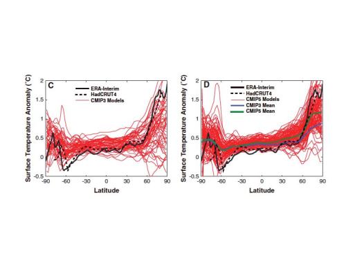
Figure 1. Changes in mean surface air temperature are the standard metric used to assess climate change. Temperature anomalies are shown for the decade 2002–2011 relative to the 1979–2001 mean. Values for the ERA-Interim reanalysis and HadCRUT4 are shown for comparison. Panel C shows these surface air temperature anomalies as a function of latitude for the CMIP3 simulations (red curves), as well as for the ERA-Interim reanalysis (heavy black curve). Panel D shows the same but for the CMIP5 simulations, with the CMIP3 and CMIP5 mean simulation curves inserted for reference.
The latitudinal structure of the warming shown in Figures 1C and 1D provides insight into the unusual behavior exhibited by the CMIP5 ensemble. In the CMIP3 ensemble, the largest deviation between observed and simulated warmings is in the Arctic, where the observed warnings are roughly 1C larger than the CMIP3 simulation ensemble mean. The CMIP5 ensemble successfully reduces this deviation in the Arctic (Figure 1D), with differences in the warming pattern between the CMIP5 and CMIP3 ensemble means outside of the Arctic consistent with diffusion of the enhanced CMIP5 warming in the Arctic into the Northern Hemisphere midlatitudes. However, the enhanced CMIP5 ensemble mean Arctic warming unveils offsetting errors in the CMIP3 ensemble mean warming (not enough warming in the Arctic, too much warming almost everywhere else), leading to the poorer overall CMIP5 ensemble mean consistency with the observed warming relative to CMIP3.
This description provides a reasonable explanation for why the CMIP5 ensemble mean performs poorly relative to CMIP3. However, the issue of the reduction in the CMIP5 simulation spread still remains. One way to approach this problem is to ask what subset of the CMIP3 ensemble has statistics most like the CMIP5 ensemble. To this end, consider a subensemble comprised of those CMIP3 simulations that warm more than the ensemble median CMIP3 simulation (hereafter CMIP3+). Curiously, the statistics of this CMIP3+ subensemble are indistinguishable from those of the CMIP5 ensemble using Student’s T-test (Table 1; p ’ 0.15 for both tropics and extratropics). This contrasts with the behavior of the entire CMIP3 ensemble, which differs from theCMIP5 ensemble in a statistically significant fashion in both the tropics and extratropics (T > 3.25; p < .002). This indicates the possibility of a selection bias based upon warming rate (either globally or regionally in the Arctic), with only those model configurations that warmed more aggressively ‘surviving’ in an appropriate sense to be included inCMIP5, while those that did not warm as aggressively were more significantly modified. This statement is of course highly speculative; the actual rationale for this convergence is likely to be more complicated.
JC comments: I find this paper to be very illuminating. The latitudinal variation of observed temperature anomalies clearly shows that most of the recent warming occurs in the Arctic. How much of the recent arctic warming is associated with external forcing (e.g. predictable) versus natural internal variability is hotly debated.
Latitudinal comparisons of climate model simulations with observations is very revealing. Climate models are not accurately simulating the hemispheric gradients in temperature anomalies, with too much warming in the lower latitudes and too little warming in high latitudes. Owing to the large multi-decadal natural internal variability in the high latitudes, the over prediction of warming in the lower latitudes may be the more telling model deficiency in terms of AGW sensitivity.
And finally, the convergence of CMIP5 models towards a common solution does give credence to Swanson’s thesis of selection bias. Gavin Schmidt is adamant that climate modelers (well at GISS anyways) don’t tune to observations. However, it is abundantly clear (see also this previous post Climate model tuning) that ‘expectations’ of model simulations do influence which model versions and combinations of parameter choices are used in the final model version for production runs.
The idea of model selection bias based on simulating a large amount of arctic warming and a sea ice decline is an intriguing one. If this is the case (again, subjective biases are not easy to unambiguously identify), then it is even more important to sort out how much of the recent Arctic warming is from AGW versus natural internal variability.

how do climate scientists deal with enthalpy?
Academia is global warming’s big loser. No one expects politicians to tell truth. But, it’s been an eye-opener for many that the teachers of climate alarmism – a self-proclaimed consensus of everyone in the government-education complex — have been so eager to succumb to bias and to blame Americanism for climate change. At the expense of truth, the facts, good rules of logic, common sense and in concert with the haters of America around the globe who have indulged in propaganda for political purposes, academics have done all they could do to bring about the fall of the country.
All society (homo sapiens) has been the loser from official deceit.
https://dl.dropboxusercontent.com/u/10640850/Creator_Destroyer_Sustainer_of_Life.pdf
The next big losers will be world leaders and the US National Academy of Sciences, the UK’s Royal Society, the UN, the National Academies of Sciences in Sweden, Norway, Germany, etc., and the publishers of textbooks and science journals that deceived the public for sixty-eight years (2013 – 1945 = 68 yrs), after the Second World War ended.
The CSALT model does enthalpy it one better. It deals with the free energy of the earth’s components. Much of the forcing that occurs is partitioned as heat and all the other terms such as pressure, wind speed, tidal energy, etc.
Applying a variational principle to free energy, the fluctuations amongst the varying energy components balance to follow the overall rise in free energy applied, which is governed by the CO2 control knob.
CSALT is a model which applies this variation approach to track the earth’s temperature. I added the free-energy contribution due to lunar tides in this post:
http://contextearth.com/2013/12/06/tidal-component-to-csalt/
‘Free energy may refer to:
In science:
Thermodynamic free energy, the energy in a physical system that can be converted to do work, in particular:
Helmholtz free energy (A=U–TS), the energy that can be converted into work at a constant temperature and volume
Work content, a related concept used in chemistry
Gibbs free energy (G=H–TS), the energy that can be converted into work at a uniform temperature and pressure throughout a system
Variational free energy, a construct from information theory that is used in Variational Bayesian methods.’ Wikipedia
One reason for disliking webby is the pretentiousness with which he approaches everything. This is very un-Australian for an honorary Australian.
This latest entry is typically heavy on terminology that means very little in terms of lucid explanations for anything he does.
The methodology he uses is an empirical deconstruction of temperature by scaling major components of climate variability to the temperature record. It is simple multiple regression – done to death in the literature and eminently ignorable. The essential problem is collinearity. My – another big word.
How much is natural decadal variability and how much is greenhouse gases. webby solves the problem in typical fashion by assuming that natural variability is negligible. More realistic analysts suggest that the proportions are indeterminate. Tung and Zhou suggest – on the basis of the CET record that it is 50%.
I have linked to this graph from Kyle Swanson and realclimate before – if anyone is counting.
http://s1114.photobucket.com/user/Chief_Hydrologist/media/rc_fig1_zpsf24786ae.jpg.html?sort=3&o=34
What does this say?
It is a simple sanity check. The warming trend is that which excludes the periods of 1976/1977 and 1998/2001 – which without going into chaos theory are extreme events at periods of climate shifts.
The residual warming – which Swanson defines as the real warming signal – is about 0.1 degrees C/decade. We can assume that at least half of that was natural variability. These decadal variations have added to and countered warming in the instrument record.
So we have some 0.05 degrees C/decade warming from greenhouse gases and this is not and never has been an existential threat in this century. Most recent warming is not greenhouse gases – quite obviously in this simple sanity check which webby (and the IPCC) persistenly fail.
Any real risk – indeterminate probability functions – comes from another quarter entirely.
‘Finally, the presence of vigorous climate variability presents significant challenges to near-term climate prediction (25, 26),
leaving open the possibility of steady or even declining global mean surface temperatures over the next several decades that could present a significant empirical obstacle to the implementation of policies directed at reducing greenhouse gas emissions (27). However, global warming could likewise suddenly and without any ostensive cause accelerate due to internal variability.
To paraphrase C. S. Lewis, the climate system appears wild, and may continue to hold many surprises if pressed.’
Swanson et al 2009 – http://deepeco.ucsd.edu/~george/publications/09_long-term_variability.pdf
Chaos is of course something else that webby fails to get.
Chief, please tell me something. Or, Web. When I read about the thermodynamic equations in differential form, it seems to me these were meant to apply instantaneously to all of a system. True, you could integrate over a time interval to get discrete changes on both sides of the equation, but the starting and ending points would be the same for all those changes. In particular, isn’t it correct to say that if the right-hand-side changes are between points t and t’ (t<t'), then the theory as written demands that the left-hand-side changes are between points t and t' and most definitely not between time points t'' and t''' where t' < t'' < t''?
I do not see how the thermodynamic equations Web uses to motivate his regressions can be anything other than a metaphor, since the right-hand-side variables are lagged some periods (months as it happens) in back of the left-hand-side variables. For an observer new to the theory but well-versed in that kind of math, it seems that these kinds of thermodynamic equations where developed to deal with "small" systems where one could regard all parts of the system as instantaneously affecting one another–not to some big, ponderous thing like a planetary system where the notion of causes preceding effects makes sense of a lag structure in the empirical implementation of the model.
Am I completely off base here, and if so, why exactly?
With Navier-Stokes we are talking about hydrodynamic continuity equations that are solved numerically on a time step and on a grid.
e.g. http://en.wikipedia.org/wiki/Navier%E2%80%93Stokes_equations
webby’s method – on the other hand – is an ’empirical decompostion’ and is peripheral to any actual physics. It is similar to the methodology of Lean and Rind.
‘From 2009 to 2014, projected rises in anthropogenic influences and solar irradiance will increase global surface
temperature 0.15 ± 0.03C, at a rate 50% greater than predicted by IPCC. But as a result of declining solar activity in the subsequent five years, average temperature in 2019 is only 0.03 ± 0.01 C warmer than in 2014. This lack of overall warming is analogous to the period from 2002 to
2008 when decreasing solar irradiance also countered much of the anthropogenic warming. We further illustrate how a
major volcanic eruption and a super ENSO would modify our global and regional temperature projections.’
So they are wrong and it is because ENSO has failed to cooperate. I suspect that ENSO will fail to cooperate with webby into the future.
e.g. http://earthobservatory.nasa.gov/IOTD/view.php?id=8703
As far as I understand, no climate model factors in the requirement from the 3rd Law of Thermodynamics that the radiation entropy production rate at ToA has always to be positive, but is minimised, and that minimisation is achieved by maximising atmospheric pCO2!
This is, of course, the mathematical theory of Gaia!
Fun to watch NW struggle with the transient simplifications of the CSALT model. It must be hard for an economist to understand the simplest of physics.
OK, here is an analogy. If I had an electrical circuit composed of inductors, capacitors, and resistors, there are many situations that I could solve the situation by assuming it was purely resistive. And then the transient stimulus response would be a slight perturbation, in which case I could model with a tuned impulse response. If it was mainly capacitive, with say only lags, the response would be purely damped, as in a low-pass filter. If you don’t like the electrical analogy replace it with dampers, springs, and mass and do a similar simplification. That is the difference between the disciplines of statics and dynamics, often referred to as a quasi-static approximation.
On the other hand, it is possible that the SOI pressure component is a complicated pseudo-resonant response function, but that is OK, because I am applying that “as is” in the CSALT model and than applying a 6 month lag to let that propagate across the world. And then when we consider that there is already a significant strong yearly oscillatory component due to the solar-influenced seasons, one realizes that it is mad to try to capture to that level anyways so we place a 12-month filter on the results..
So the proof is in the pudding and you will have to explain why CSALT works so well to explain what it does.
Why does it infer the strength of the TSI component correctly?
Why does it get the phase of and strength of the tides so accurately?
Why does it explain the 60-year pseudo-cycle using the Stadium Wave LOD so well?
Why does it explain the long pause starting in the 1940’s extending to the 1970’s so well?
Why does it explain the most recent pause so well?
Why does it tune to the orbital pseudo-cycles of Scafetta so well?
Why does it explain the measurement anomalies around WWII so well?
Why doesn’t it do something stupid, like invert the sign of the aerosol functions?
Why is it robust against using different data sets, such as GISS versus NRDC versus HADCRUT?
and finally
Why can’t any skeptical model touch it?
Because CO2 is the control knob that controls the long-term climate, that’s why. And every skeptical model is ABCD and automatically loses.
“So the proof is in the pudding and you will have to explain why CSALT works so well to explain what it does”
Degrees of freedom
One might also note that entropy and enthalpy are descriptive fictions that we use to describe a system, they do not actually exist. Matter does not decide if what it is doing is going up or down hill, on any scale.
Doc, Degrees of freedom don’t count if they are based on actual physical parameters. Is the speed of light at 3e8 m/s a degree of freedom? Is the force of gravity at 9.8m/s^2 a degree of freedom? Is the lunar nodal period of 18.6 years a degree of freedom? Using data from other observational sources is also not as strong a degree a freedom as using model parameters. So when I use the SOI pressure difference, this is not necessarily a degree of freedom in the statistical sense. It actually exists in the free energy variational decomposition of the system. The CSALT model is simply figuring out what the strength of these individual factors are.
So when CSALT can figure out the tidal contribution of the temperature trend as well as it does
http://contextearth.com/2013/12/06/tidal-component-to-csalt/
then it becomes less a degree of freedom than it is a description of the free energy contribution.
I can name the significant degrees of freedom as I see it. One is the lag on the LOD Stadium Wave component, which is about 5 years. Another is the individual contributions of the volcanic forcings, as these need to be estimated In the CSALT model, I only take the volcanic eruptions that are greater than 4 on the Volcanic Explosivity Index scale, except for 2 that occurred before 1900. These 10 VEI=5 or VEI=6 events have very precise timings so that they are highly tunable.
Other than that, the degrees of freedom argument is sour grapes. I am using the data that Scafetta, Curry, Bob Carter, Clive Best, Dr. Norman Page (suggesting It’s the Sun, Stupid), and other smart skeptics suggest using and now it is not so good because CSALT works so well. Too bad.
So the proof is in the pudding and you will have to explain why CSALT works so well to explain what it does.
OK. Let’s have at it.
Why does it infer the strength of the TSI component correctly?
Because if it did not it would not be published.
Why does it get the phase of and strength of the tides so accurately?
Because the phase and strength of past tides are known at the time the model is run.
Why does it explain the 60-year pseudo-cycle using the Stadium Wave LOD so well?
Because if it didn’t it would not have been published.
Why does it explain the long pause starting in the 1940′s extending to the 1970′s so well?
Because if it didn’t it would not have been published.
Why does it explain the most recent pause so well?
Note the use of the word “explain.” It did not predict the pause
.
Why does it tune to the orbital pseudo-cycles of Scafetta so well?
Because if it did not it would not have been published.
Why does it explain the measurement anomalies around WWII so well?
Because if it did not it would not have been published.
Ah, I give up. I cannot understand why it is a mystery to people who ought to know better that the ability of a model to predict past measurements is not necessarily indicative of the strength of the model. Explaining past data is necessary but not sufficient to validate a model.
When the model correctly predicts something unexpected in the future, then it will be (more) validated. Validation on past data is simply not acceptable science. There are many, many historical examples of unconscious bias introduced into models and even measurements. Take a look, for example, at the history of measurements of the speed of light. Or take a look at physics codes used to model plasmas.
Web, since your (alleged) theoretical justification comes from taking a total differential of a definition of Gibbs energy, wouldn’t it be most sensible to do your estimation on first differences rather than levels? When I do that using your data, using just march and september observations, the resulting R-squared is about 0.15 (not the roughly 0.85 you get) and the estimated coefficient on lagged change in co2 is about 6 with a standard error of about 11… that is, noisy as all get-out and so insignificantly different from zero. (To be clear, I have only used the three right-hand-side variables that you use at a 6-month lag, so that the lag structure matches the differencing structure.)
Is there a reason your variational approach should crash and burn in first differences while appearing to be so very swell and dandy in levels? I mean a physical reason.
“wouldn’t it be most sensible to do your estimation on first differences rather than levels? ”
No.
‘
Obviously you did something wrong (R).
Your own interpretation of the variational approach crashes and burns.
Why not start with a quasi-static approach? Because of the difficulty of taking any derivatives of less than a year or of dT’s that span parts of years, you won’t get anywhere.
Argument from assertion does not cut it. Find something actually wrong with what I am doing, not something that you dream up based on what someone else has done. You sound like a Luddite.
eb, I easily replicate the regression you have with the (6 6 6 24 60)-month lag structure. I’m not making a mistake.
If this equation is right…
T(t) = B’X(t-lxi)
where B is a vector of coefficients, X = (x1,x2,..xi,…xn) is a vector of regressors, and lxi is your lag length for regressor i,
Then this equation is also right (if, as you have claimed, time series data issues are irrelevant to estimating your model):
DT(t) = B’DX(t-lxi)
Here the D operator is a six-month first difference, that is,
DY(t) = Y(t) – Y(t-6).
I choose march and september because fixed effects for march and september are the closest to zero for two months separated by six months, in a regression of T on month effects and a cubic in t. In other words, differences between september and march (or vice versa) don’t show an intra-annual pattern.
NW, this isn’t econometrics.
Web, neither was that post.
No one is looking at sub-yearly resolution with this.
Then, in what sense is a 6-month lag from co2 impulse to temperature response meaningful? For that matter, why use monthly data at all? If you are claiming that the co2 signal is invisible in high frequency time series, why use a high frequency time series? Because it builds up (strictly phony, because of autocorrelation) degrees of freedom?
You should watch Trenberth’s recent video. He said the biggest contribution to climate is the seasonal cycle. If one considers that alone, the climate sensitivity has to be at least 3C for a doubling of CO2.
The reason that I am using monthly is because I want to make sure all the time series are accurately aligned with one another. But not all of the time series are given by monthly values, and some are given as yearly averages. So where does a year’s value kick in — halfway through that year? That’s why it is nice to be able to line these up using a subyear resolution. I also use an interpolation scheme for data that is only yearly. The last thing I am going to do is throw out monthly data if that is available.
BTW, a six-month lag has tails that extend beyond a year, I hope you realize.
Another thing about the Trenberth presentation video, he says that “with all the economists here, I have to talk about the real system”.
Too funny and so true!
With clouds (http://judithcurry.com/2012/11/28/clouds-and-magic/), ocean cycles (http://judithcurry.com/2013/08/16/climate-model-simulations-of-the-amo/) and solar cycles (http://judithcurry.com/2013/10/01/ipcc-solar-variations-dont-matter/) modeled poorly, if at all, it is all the more disturbing that policymakers rely on climate models to justify sweeping economic and social policies.
how much of the recent Arctic warming is from AGW versus natural internal variability.
The Vikings moved to Greenland and the Chinese sailed to the North Pole because the same natural Variability that we have now was in place then.
no the chinese did not sail to the north pole
No the Chinese did not sail to the North Pole.
And you know this, how?
Someone mapped the world between 1400 and 1500.
Who made the maps?
No other country had enough ships and resources to map the whole Earth at that time.
Offer your alternate theory[s]
I guess it would follow, from your view, that the Vikings did not live in Greenland because Earth was not as warm as history records.
Or, Greenland got warm, but it had nothing to do with warmer oceans that also opened the Arctic.
Or, the hockey stick is right and the Warm Periods in the historic past never happen.
China was well ahead of the west in its technical ingenuity
before 1400. The Chinese invented the compass and were
clever map makers. In the years, 1405-1430 the admiral,
Zheng He supervised major visits to distant lands by large
‘treasure ships.’ Under the new Emperorer the ships were
allowed to rot in the harbour.
According to Wiki, treasure ships were accounted to be in
use in the Song Dynasty, 960 -1279. May have sailed north
… or not.
The Chinese may have sailed up to the North Pole without telling anyone about it. That would explain why there are no records of them having been there.
Today tomatoes and strawberries are grown in Iceland, which means it’s warmer there now that it was during the MWP because the Vikings back then didn’t grow those things.
I meant to say tomatoes and strawberries are grown today in Greenland.
On the permafrost?
Tomatoes are a New World crop (from Mexico). Strawberries have to be grown in a climate-controlled greenhouse, and I think those first appeared in 1450.
I meant to say that the Iceland strawberries are grown in greenhouses. I don’t know about the Greenland ones.
Nice one Max_OK
Here are some more details of the Chinese world mapping
http://www.chengho.org/news/chinesemap.php
What’s next? aliens built the pyramids?
No, they provided a blueprint and cloned army of slaves for the donkeywork.
The specific differences from what was modeled are interesting, but it does not seem at all unexpected. There was such a low confidence in any individual model that they resorted to the use of a model ensemble of unknown quality to form conclusions.
The specific differences from what was modeled are interesting, but it does not seem at all unexpected. There was such a low confidence in any individual model that they resorted to the use of a model ensemble of unknown quality to form conclusions.
And this is a big problem. It has been quite apparent of late that the climate science community is using the variance of model ensembles as a kind of surrogate for experimental error bars. That such a use is entirely wrong should be obvious to any second-year statistics student. This fact causes me a great deal of concern about the average competence of the climate community’s use of statistics.
In particular, the use of common elements between models in the ensemble mean that the variance between models is nowhere near stochastic, as seems to be commonly assumed. Selection bias makes the problem a great deal worse.
What’s really frustrating about this problem is that it’s just math. It’s not rocket science or (my field) nuclear physics. Math should always be done correctly in a published paper. Yet we’ve seen many examples of embarrassingly incorrect statistics published by so-called luminaries in climate science (Michael Mann, anyone?) and staunchly defended by others in the same field.
There is, quite simply, no excuse for getting basic statistics wrong.
fizzy
The unspoken excuse is “the ends justify the means”. Ends include saving the planet from too many people, saving the gravy train of research funding, saving the gravy train of green energy initiatives, and political power over private energy markets.
Judith writes: “Latitudinal comparisons of climate model simulations with observations is very revealing.”
For years, I’ve been showing model failings using latitudinal trends. The models look even worse when sea surface temperature data are isolated from land surface temperature data.
Globally since Nov 1981:
http://bobtisdale.files.wordpress.com/2013/11/figure-7-2.png
Or if you’d prefer, the Atlantic:
http://bobtisdale.files.wordpress.com/2013/02/03-zonal-atlantic.png
The Indian:
http://bobtisdale.files.wordpress.com/2013/02/04-zonal-indian.png
And one of my favorite model-data comparisons, the Pacific:
http://bobtisdale.files.wordpress.com/2013/02/02-zonal-pacific.png
The ocean-basin graphs above are from my most recent sea surface temperature model-data comparison:
http://bobtisdale.wordpress.com/2013/02/28/cmip5-model-data-comparison-satellite-era-sea-surface-temperature-anomalies/
Just about time for an annual update.
And the global comparison is from the book “Climate Models Fail”:
http://bobtisdale.wordpress.com/2013/09/24/new-book-climate-models-fail/
Regards
every Climate Modeler has a Ph D in Cherry-Picking – trust them…
As fig leaves go, that one is a bit too small.
All models use CO2 warming to drive (“force”) climate developments. If this assumption is wrong, no model selection, biased or otherwise, will produce a subensemble that performs any better than the originals
When Models fail to show skill for 17 years, some important basic assumption must be wrong.
Ice Extent and Clouds adjust the Albedo of Earth. CO2 is here to make the green stuff grow.
Temperature always goes up when Albedo goes down and always goes down with Albedo goes up.
Consensus Theory adjusts Ice Extent and Albedo as a result of feedbacks they can’t explain.
They have it backwards. Albedo changes and adjusts the temperature. It really is this simple.
Ewing and Donn, 1950’s
‘Lorenz was able to show that even for a simple set of nonlinear equations (1.1), the evolution of the solution could be changed by minute perturbations to the initial conditions, in other words, beyond a certain forecast lead time, there is no longer a single, deterministic solution and hence all forecasts must be treated as probabilistic. The fractionally dimensioned space occupied by the trajectories of the solutions of these nonlinear equations became known as the Lorenz attractor (figure 1), which suggests that nonlinear systems, such as the atmosphere, may exhibit regime-like structures that are, although fully deterministic, subject to abrupt and seemingly random change.’
http://rsta.royalsocietypublishing.org/content/369/1956/4751.full
There are multiple solutions for any model. Effectively in the order of hundreds. A single solution derives from a combination of attributes including coupling breadth and parametisation of uncertainties. Changing the attributes slightly can change the solution radically – as Lorenz discovered.
e.g. http://rsta.royalsocietypublishing.org/content/369/1956/4751/F8.expansion.html
Selection of a single solution from hundreds of potential – and divergent – solutions is inevitable unless the results are reported as probabilities. There is no valid methodology for distinguishing between solutions.
I have an idea that couplings and parameters are determined on the basis that they provide a ‘plausible’ solution – i.e. warming in a certain range. Trial solutions – try a particular combination of feasible couplings and parameter values and if it gives a plausible solution – it must be right.
‘AOS models are therefore to be judged by their degree of plausibility, not whether they are correct or best. This perspective extends to the component discrete algorithms, parameterizations, and coupling breadth: There are better or worse choices (some seemingly satisfactory for their purpose or others needing repair) but not correct or best ones. The bases for judging are a priori formulation, representing the relevant natural processes and choosing the discrete algorithms, and a posteriori solution behavior.’
http://www.pnas.org/content/104/21/8709.long
Emphasis added in both cases. If solutions can only be understood in terms of probabilities – they need to take the next step of perturbed physics models.
‘A more comprehensive, systematic and quantitative exploration of the sources of model uncertainty using large perturbed-parameter ensembles has been undertaken by Murphy et al. [24] and Stainforth et al. [25] to explore the wider range of possible future global climate sensitivities. The concept is to use a single-model framework to systematically perturb poorly constrained model parameters, related to key physical and biogeochemical (carbon cycle) processes, within expert-specified ranges. As in the multi-model approach, there is still the need to test each version of the model against the current climate before allowing it to enter the perturbed parameter ensemble. An obvious disadvantage of this approach is that it does not sample the structural uncertainty in models, such as resolution, grid structures and numerical methods because it relies on using a single-model framework.
As the ensemble sizes in the perturbed ensemble approach run to hundreds or even many thousands of members, the outcome is a probability distribution of climate change rather than an uncertainty range from a limited set of equally possible outcomes, as shown in figure 9. This means that decision-making on adaptation, for example, can now use a risk-based approach based on the probability of a particular outcome.’
http://rsta.royalsocietypublishing.org/content/369/1956/4751.full
Chief
“There is no valid methodology for distinguishing between solutions.”
Does this mean that all solutions should be treated as “plausible”? If so, is it plausible that “cooling” solutions should be considered as well?
If radiative physics are intrinsic to current models, and cooling is within the plausible solutions, do we suggest that radiative physics “warming” may not be an important parameter.
If one cannot distinguish between solutions, aren’t there even more solutions than those that contain radiative physics?
Lorenz entered truncated parameters into his convection model – 3 instead of 6 decimal places – in the expectation that it would make very little difference in the output. He was wrong and discovered metaphorical butterflies. Climate models are undoubtedly chaotic given the underlying nature of the Navier-Stokes PDE. Make a small change in inputs and the potential for large changes in outputs is there necessarily and unpredictably. In any model there is a range of feasible parameters, coupling and parametisations that introduce instability into the calculation. As James McWilliams said.
‘Sensitive dependence and structural instability are humbling twin properties for chaotic dynamical systems, indicating limits about which kinds of questions are theoretically answerable. They echo other famous limitations on scientist’s expectations, namely the undecidability of some propositions within axiomatic mathematical systems (Gödel’s theorem) and the uncomputability of some algorithms due to excessive size of the calculation (see ref. 26).’ http://www.pnas.org/content/104/21/8709.long
The precision and quantity and selection of measurements used to prime or assess models falls well below the “truncation” sensitivity boundary that spund Lorenz’ models into unpredictability. It is perverse and presumptuous to assume current models have anything useful to tell us whatsoever.
Count, e.g., the number of significant digits of historical temperature records, to start. Even if recorded on the full Kelvin scale, it rarely exceeds 3.
spund = spun
If radiative physics are intrinsic to current models, and cooling is within the plausible solutions, do we suggest that radiative physics “warming” may not be an important parameter.
IR does supply most of the cooling for Earth, but it has no Set Point. The Polar Sea Ice Extent does the fine tuning of temperature.
As the ensemble sizes in the perturbed ensemble approach run to hundreds or even many thousands of members, the outcome is a probability distribution of climate change rather than an uncertainty range from a limited set of equally possible outcomes, as shown in figure 9. This means that decision-making on adaptation, for example, can now use a risk-based approach based on the probability of a particular outcome.
That statement is so wrong on so many levels I don’t even know how to begin. The fact that this paper was even published boggles the mind.
An ensemble of chaotic predictions from a model can only approximate a probability distribution of observables if the model is perfect. Systematic effects (e.g. model imperfections) introduce systematic biases in the model outputs, which can no longer be treated as probabilistic representations of some true distribution.
What is done in climate science is even worse: ensembles of different models are combined and treated as probability distributions. The justification appears to be an intuitive belief that the systematic errors in the various models will obey the central limit theorem and tend to average out. Unfortunately, that would require several factors that are not present.
The observed bias in publication rates for models based on predicted warming means that almost certainly the “probabilistic” estimate of warming that one gets from an ensemble will be too high, even if no single researcher is attempting to bias the results.
Like I said before, it is just math. Its not a matter of opinion.
Because most of the world’s heat is generated in the Northern hemisphere we would expect the Arctic to be warmer than the Antarctic. Global average temperature is something of a fiction because it has to be calculated from many sensors, with too many in some areas and too few in others.
I have looked at the CLIVAR web site and it seems to reflect their ambitions, although there are problems
(a) Like the IPCC they have ignored global temperature change pre-1960,
and
(b) the quality of rendition of graphs on their website is so bad as to be: almost unreadable even with the help of the magnifier app.
“Global average temperature is something of a fiction because it has to be calculated from many sensors, with too many in some areas and too few in others.”
“they have ignored global temperature change pre-1960”
Don’t forget that pre-1960 global temperature change has to be calculated from many sensors, with too few in some areas. So I have no idea what fictional pre-1960 changes you are talking about.
So you don’t see a difference between global average temperature and global temperature change?
Arctic warming has nothing to do with heat generation in the northern hemisphere, It has to with no continent covering the north pole giving the ocean conveyor belt the opportunity to extend circulation of tropically heated water all the way to the north pole. Anthropogenic heat is insignificant in comparison to total surface energy budget except in urban heat islands and those are miniscule in comparison to total surface area.
lolwot: Thank you for your reply. In areas where there are too few sensors, like the polar regions, the gaps have to be filled by some sort of spatial (and maybe temporal) interpolation formula. That is why the results are somewhat artificial. This is not a criticism of the technique.
Early 20th century temperature records are important because they gave the first solid evidence of anthropogenic climate change. And most intriguing in 1940 was the complete stoppage and rapid reversal of temperature change. This has never been explained. Had the IPCC tried to explain this, they would have realized that no continuous differential equation style model would work. This was on/off climate change like a switch. Nothing in nature like this except in quantum mechanics. See the BOM graph in my figure underlined above.
David: thanks for your remarks. If the conveyer belt continues under the polar ice, it would have little effect on temperature because the thick polar ice would be such an efficient insulator. One would expect the warmish salt laden water to gravitate into the deepest trenches first.
When all you have is CO2, everything appears as a temperature delta.
I quote “and corresponding decline in Arctic sea ice.”
It seems to be that there is an inherent assumption in this study, that Arctic sea ice is on an unequivocal long term decrease in area; presumably caused by CAGW. I am watching the current refreeze of the Arctic sea ice, and it seems to me that it has all the characteristics of a recovery to the sort of extent that existed to that when satellite images first became available. That was about 40 years ago, and one cannot expect this recovery to take place in a few years. But, to me, the signs are that the variations in sea ice, together with surface temperatures, are cyclical, not inexorably in one direction, albeit with noise.
I am somewhat interested in what many climate scientist will say if we note an increase in ice extent for a prolonged period of time.
Doc
Global climate disruption. They floated the phrase a few years ago in anticipation.
Extreme and sudden change characterize the transitions between glaciation and deglaciation. If, in fact, climate is disrupted, it might be signaling the end of the Holocene. Fortunately, observations tend not to show contemporary extremes. Whew!
======================
Arctic ice increased a third over last year I believe, while antarctic has the greatest extent in over 30 years. Globally, no additional warming in 17+ years. No increased trends in hurricanes or tornadoes.
Meanwhile, the L.A. Times has banned all letters that dare question AGW and in Boston they’re calling for Jeff Jacoby’s head for writing a skeptical newspaper column.
Somebody wake me up. I must be having a bad dream.
Say, pokerguy, that ‘which may not be questioned ..’
er.. may not be questioned. (
Statistically, it is impossibly hard to discern underlying trends amidst so much noise. So hard, if fact, that it’s impossible for climate alarmists to claim otherwise and remain credible. Only a desire-driven bias cuts through the deafening cacophony of natural variability to arrive at the conclusion that the actions of humanity are driving weather and by extension climate change.
The doubt that may not speak its name, Dear Beth.
“no additional warming in 17+ years”
The trend over the last 17+ years is positive. You can’t claim there’s been no additional warming when the error bars cover warming.
How many times do me and others have to set you guys straight?
lolwot speaks the truth. I know because I looked at the facts.
http://www.woodfortrees.org/plot/hadcrut3vgl/from:1996/plot/hadcrut3vgl/from:1996/trend/plot/gistemp/from:1996/plot/gistemp/from:1996/trend/plot/uah/from:1996/plot/uah/from:1996/trend/plot/rss/from:1996/plot/rss/from:1996/trend/plot/none
“How many times do me and others have to set you guys straight?”
Mostly just you, Lolly. But carry on. Always entertaining.
Remember when things like statistical significance and global average surface temperatures mattered in climate “science”?
The trend over the last 17+ years is positive. You can’t claim there’s been no additional warming when the error bars cover warming.
So, there has been no additional warming that is supported by actual data. Only error bars. And we have 17 years of data on the Error Bars that grow every year.
Does GaryM know about Type 1 and Type 11 errors? I’m not sure I know which is which.
Anyway, if in a year’s time a 5-year old child’s height increased, but the increase wasn’t statistically significant, and we concluded the kid could look forward to a career in a carnival side show, would we be committing one of those errors?
Type I and II errors are false positives and false negatives respectively.
Unless you take on board the idea of climate shifts – e.g. http://www.sciencedaily.com/releases/2013/08/130822105042.htm – you don’t have a clue about climate and any analysis is based on incorrect theory.
Take into account climate shifts and you can begin to understand why temperature has not trended down since the last climate shift (1998/2001) and why increases seem unlikely for the next 10 to 30 years.
http://www.woodfortrees.org/plot/hadcrut4gl/from:1998/plot/hadcrut4gl/from:2002/trend:2002
whoops… has trended down since 2002…
Chief Hydrologists said “Take into account climate shifts and you can begin to understand why temperature has not trended down since the last climate shift (1998/2001) and why increases seem unlikely for the next 10 to 30 years.”
_____
Sure you can predict what will happen in the next 10 to 30 years by looking at historical patterns. You can also do it by
looking at tea leaves or chicken entrails.
BUT the taste of the pudding is in the eating. If contrary to your prediction, the average global temperature increases for the “next 10 to 30,” your pudding is going to taste like crow. Of course, you may be senile by then, not remember what this is about, and deny ever making such a prediction.
To quote myself. Anastasios Tsonis, of the Atmospheric Sciences Group at University of Wisconsin, Milwaukee, and colleagues used a mathematical network approach to analyse abrupt climate change on decadal timescales. Ocean and atmospheric indices – in this case the El Niño Southern Oscillation, the Pacific Decadal Oscillation, the North Atlantic Oscillation and the North Pacific Oscillation – can be thought of as chaotic oscillators that capture the major modes of climate variability. Tsonis and colleagues calculated the ‘distance’ between the indices. It was found that they would synchronise at certain times and then shift into a new state.
It is no coincidence that shifts in ocean and atmospheric indices occur at the same time as changes in the trajectory of global surface temperature. Our ‘interest is to understand – first the natural variability of climate – and then take it from there. So we were very excited when we realized a lot of changes in the past century from warmer to cooler and then back to warmer were all natural,’ Tsonis said.
Four multi-decadal climate shifts were identified in the last century coinciding with changes in the surface temperature trajectory. Warming from 1909 to the mid 1940’s, cooling to the late 1970’s, warming to 1998 and declining since. The shifts are punctuated by extreme El Niño Southern Oscillation events. Fluctuations between La Niña and El Niño peak at these times and climate then settles into a damped oscillation. https://quadrant.org.au/opinion/doomed-planet/2010/02/ellison/
So looking in detail at patterns of variability in ENSO is the same as reading tea leaves? In general Max has even less knowledge than numbnut – much less than webby although the latter is pretty much the dark side of intellectual endevours – and revels in his ignorance. He doesn’t need any stinkin’ book learnin’. Really – Max seems the utter dregs of the climate war. Both a lack of knowledge and a lack of integrity.
His gratuitous, unwelcome, ignorant and frankly idiotic discussion of senility is merely another example of disingenuous obfuscation. It has nothing to do with science of course – more Allinsky then Einstein.
And if it goes the other way?
Some will never understand – some will take the Kool-Aid option.
Let me be clear – this is not a prediction. PDO and ENSO are solidly in the cool mode and the AMO is trending down. These modes last 20 to 40 years. It is the climate equivalent to saying today is Saturday – all day long.
pokerguy | December 6, 2013 at 10:39 pm |
“How many times do me and others have to set you guys straight?”
Just one time. But you have it straight yourself first. Therein lies the rub. :-)
We already know with high confidence that the globe has warmed over the last 17 years. Apart from ocean heat content increasing, even global temperature when corrected for ENSO shows an increase. See Web’s CSALT model for example. Global temperatures that used to require El Nino are now being brought about by ENSO neutral alone.
And we must not forget to factor in the tiny, yet significant cooling from the quiet Sun (and according to some the negative PDO too).
All this evidence leads to high confidence that the world has continued warming for the last 17 years.
Further, given the high confidence that natural forcings have had a cooling influence in the last 17 years, this also gives confidence that the cause of the warming in the last 17 years is anthropogenic.
The only serious question is how bad the anthropogenic warming will turn out to be, ie how much of it has been masked by the natural cooling. Those (skeptics) who exaggerate tenuous PDO and solar cooling theories actually have more reason than us realists to believe the human warming is worse than thought. Afterall if the Sun and negative PDO have caused 0.2C cooling since 1997 and yet the HadCRUT trend since 1997 is positive, what does that say about the human driver?
Still a mystery why some people call themselves skeptics.
http://wottsupwiththatblog.files.wordpress.com/2013/12/arcticice.png?w=1200
Interesting that PG would pick 2003 as a point of comparison, isn’t it? Selection bias in PG”s modeling might be the explanation.
Perhaps if trying to discern trends, it might make sense to look at time frames longer than one year?
lolwot, you write “After all if the Sun and negative PDO have caused 0.2C cooling since 1997 and yet the HadCRUT trend since 1997 is positive, what does that say about the human driver?”
Your logic is superb, and I cannot refute it. All I would point out is that you have nailed your colors to the mast of an imminent rise in global temperatures, and ocean heat content. Mother Nature is a bitch. It will be interesting to see what excuses you and all the rest of the warmists come up with, when, as the proper science indicates, global temperatures continue to cool, and probably at an increasing rate, for the rest of this century.
“when, as the proper science indicates, global temperatures continue to cool”
You mean proper science like the UAH satellite record that shows a positive warming trend?
Or not that?
Re phatboy’s post on December 7, 2013 at 3:33 am |
phatboy quotes me from my comment to Chief Hydrologist: “If contrary to your prediction, the average global temperature increases for the “next 10 to 30,” your pudding is going to taste like crow. Of course, you may be senile by then, not remember what this is about, and deny ever making such a prediction.”
Then phatboy asks: And if it goes the other way?
_______
Well, the Chiefs prediction would be no more accurate than the same prediction I made by reading tea leaves, although it would be repeatable while the tea leave readings wouldn’t be (not likely anyone would read them the same way)
By buying into the climate shift thing as a predictor, Chief assumes global temperature change is simply a function of time, with temperature being the dependent variable and time being the independent variable. Of course temperature change is not simply a function of time. If it were, we could just extrapolate a least squares line and have an dependable forecast of temperature centuries into the future.
lolwot, you write “You mean proper science like the UAH satellite record that shows a positive warming trend?”
Over how many years back from the present, November 2013?
Buying into climate shifts?
In the next thread Trenberth and Fasula discuss the nature of the cooling. It includes natural decadal variation from these shifts at decadal scales.
These natural decadal variations persist for 20 to 40 years. It is clearly not a matter of projecting temperature as such but understanding at a fundamental level the nature of the system.
Climate is fundamentally deterministically chaotic and thus in principle – unpredictable. But the climate shift happened in 1998/2001 – e.g. http://www.sciencedaily.com/releases/2013/08/130822105042.htm – and thus is the antithesis of prediction.
The globally averaged temperature doesn’t change unless there is a forcing applied. All the ENSO forcings revert to the mean, and so all that is left is the long-term upward warming trend provided by the CO2 control signal.
WHUT, you write ” and so all that is left is the long-term upward warming trend provided by the CO2 control signal”
What “CO2 control signal”? No-one has ever measured a CO2 signal in any modern temperature/time graph.
The one that we can infer, like we can infer the role of the moon in tides.
And to top that off, the role of tides that we can infer in subtle temperature shifts
http://contextearth.com/2013/12/06/tidal-component-to-csalt/
Crip, it must be hard for you when you have lost your physics touch.
WHUT, you write “The one that we can infer, like we can infer the role of the moon in tides.”
Sheer and utter nonsense. Complete scientific garbage. There are centuries of empirical data which gives us a complete understanding how gravity affects things, even though we may not know why gravity exists.
There is no empirical data whatsoever to show that a CO2 signal exists at all; zero, nada, zilch. There is simply no empirical data whatsoever for a scientific basis on which to establish that additional CO2 has any affect on global temperatures at all.
You are operating on the basis of hypotheses and meaningless estimations.
Crip, it must be tough on you when all you can do is needlepoint.
WHUT, you write “Crip, it must be tough on you when all you can do is needlepoint.”
A very sincere “thank you”, for that response. I come onto blogs for my own education; bouncing ideas off very knowledgeable people. My responses to you were all just science. The best you can come up with is a snide remark about what I like to do for pleasure. And you even go this wrong. I don’t do needlepoint; I do counted cross-stitch.
You confirm that the science, physics, I have written is, basically, correct.
Crip, If you were in it for the science, instead of just passing the time, you would be doing the kind of analysis that I am doing.
Can you do this in cross-stitch?
http://imageshack.com/a/img577/8173/6pu.gif
WHUT, you write “Can you do this in cross-stitch?”
Yes, I could do it in counted cross stitch. But it is very uninteresting, and I would not want to. CSALT is an excellent exercise in curve fitting using a number of parameters, but it as no utility in foretelling the future, until it has been validated. It reminds me of Hasting’s Approximations for Digital Computers.
Better pack it in then Crip
An extra great zinger in the CSALT model is that it is an example of a great heuristically-based estimating tool, even if somebody doesn’t understand the physics. Generating a fit with R=0.994 and with that kind of yearly resolution over the past 130+ years is not easy to do.
So in terms of heuristics, one can then plug in the parameters to CSALT which can be projected, such as future CO2, TSI, and orbital cycle values and then guess as to the extents of SOI and volcanos, and you have a useful climate projection tool.
Too bad Crip doesn’t understand that heuristics are never validated. As long as they work, people will use them.
It must pain him to no end.
“Gavin Schmidt is adamant that climate modelers (well at GISS anyways) don’t tune to observations”
THE PHYSICS THAT WE KNOW
A Conversation with Gavin Schmidt
‘It turns out that the average of these twenty models is a better model than any one of the twenty models. It better predicts the seasonal cycle of rainfall; it better predicts surface air temperatures; it better predicts cloudiness. This is odd because these aren’t random models. You can’t rely on the central limit theorem to demonstrate that their average must be the best predictor, because these are not twenty random samples of all possible climate models.
Rather, they have been tuned and they have been calibrated and they have been worked on for many years in trying to get the right answer. In the same way that you can’t make an average arithmetic be more accurate than the correct arithmetic, it is not obvious that the average climate model should be better than all of the other climate models. For example, if I wanted to know what 2+2 was and I picked a set of random numbers, averaging all those random numbers is unlikely to give me four.
Yet in the case of climate models, this is kind of what you get. You take all the climate models, which give you numbers between three and five, and you get a result that is very close to four. Obviously, it’s not pure mathematics. It’s physics, it’s approximations, it involves empirical estimates.. But it’s very odd that the average of all the models is better than any one individual model.’
http://edge.org/conversation/the-physics-that-we-know
Modeling an Abrupt Climate Change
By Allegra LeGrande and Gavin Schmidt — January 2006
‘ The spread in model projections for the North Atlantic MOC as a function of increasing greenhouse gases is extremely large, ranging from an almost 50% decrease to a small increase by 2100. In part, this uncertainty stems from modellers tuning for the existence of a stable North Atlantic circulation, but not being able to tune for its sensitivity for lack of appropriate data.
http://www.giss.nasa.gov/research/briefs/legrande_01/
His ball.
Although clear word choices would be nice, in the end I don’t care if they tune their models so that some of their parameters match some function of observed sample moments in some training sample. Heck, I do that all the time. But I do care if they don’t appropriately propagate the sampling variability of those sample moments through their models to their forecasts (or projections, or whatever they want to call them).
It turns out that the average of these twenty models is a better model than any one of the twenty models.
It really turns out that these are really Curve Fits and have little to do with actual models.
NW. All the models are right a lot of the time and terribly wrong a small amount of the time. Averaging them yields an ensemble that is a little wrong all the time. Hence the ensemble prediction of global average temperature has gradually drifted away from actual GAT. After 20 years the accumulated small error has pushed the ensemble prediction outside the 95% confidence bound. Not surprisingly to the well-informed objective observer of climate change hysteria amongst the climate science boffins and sycophants the model ensemble erred on the warming side. Catastrophic warming is actually beneficial warming.
You would be well served to write that down.
‘Prediction of weather and climate are necessarily uncertain: our observations of weather and climate are uncertain, the models into which we assimilate this data and predict the future are uncertain, and external effects such as volcanoes and anthropogenic greenhouse emissions are also uncertain. Fundamentally, therefore, therefore we should think of weather and climate predictions in terms of equations whose basic prognostic variables are probability densities ρ(X,t) where X denotes some climatic variable and t denoted time. In this way, ρ(X,t)dV represents the probability that, at time t, the true value of X lies in some small volume dV of state space.’ (Predicting Weather and Climate – Palmer and Hagedorn eds – 2006)
Model trajectories are radically different – each solution varies by quite a lot. It seems unlikely therefore all of the models are correct most of the time.
The differences are better understood in terms of irreducible imprecision –
‘Simplistically, despite the opportunistic assemblage of the various AOS model ensembles, we can view the spreads in their results as upper bounds on their irreducible imprecision. Optimistically, we might think this upper bound is a substantial overestimate because AOS models are evolving and improving. Pessimistically, we can worry that the ensembles contain insufficient samples of possible plausible models, so the spreads may underestimate the true level of irreducible imprecision (cf., ref. 23). Realistically, we do not yet know how to make this assessment with confidence.’
http://www.pnas.org/content/104/21/8709.long
Jabberwock doesn’t even have to write it down – it is in the peer reviewed literature.
Dear Chief Kangaroo Skippy Hyperbologist Ellison,
We are supposed to be entering a kindler, gentler Climate Etc. commentary period. In the interest of complying with our lovely gracious hostess I would ask that you cease the name calling.
Kind Regards,
Jabberwock
Since Joshua has not arrived yet, I’ll play his part: What about the selection bias in selecting to post this article. :)
On a more serious note, I suspect that Gavin’s claims about not tuning the models is “true”. However that may be only because they already tuned them over the last 20 years and now know what starting parameters to give the programs so they are already pre-tuned.
There’s more than one way to tune a model, Bill. The observations can be tuned to match model outputs as well as model outputs being tuned to match observations. There’s a lot of both with increasing observation tuning with increasing temporal distance into the past. Our instrumentation is increasingly inadequate the farther back in time you go and so the opportunities for massaging the data (selection bias) increase the farther back in time you go. In one notorious case going back a thousand years or so the global average temperature record is taken from the width of tree rings in just several isolated cherry-picked trees. In the more recent period when the tree ring data could be checked against thermometer data and was found to be in disagreement the usual suspects simply stopped using the tree ring data circa 1960 and quietly stiched in the thermometer data which most scientists, under normal circumstances, would categorize as scientific fraud. See here for the full story:
Classic “Kennel Blindness” …But then,Mother Nature is a B1tch…
so it may be DNA…
Selection bias? Or data tampering? There are potentially many reasons the models do not work. But as long as new research is suppressed, and data and methods hidden, the biases will continue.
conspiracy theories?
Which ones are you espousing? I merely stated facts.
The vast majority of bias is not deliberate and this almost certainly applies to all areas of science, including climate science. People tend accept things going the way they think they should go and question things that go the way they don’t expect.
My mentor told me a great story about his Ph.D. supervisor, David Keilin
http://en.wikipedia.org/wiki/David_Keilin
Keilin had purified some beef liver catalase and wanted to make the fluoride complex. He took a bottle of sodium fluoride, put a mg on the end of a spatula, then mixed it in a cuvette of catalase solution. He held it to the light, didn’t see the color change, and so poured the NaF down the sink, flushed it away and commented ‘It’s gone off’.
How does NaF ‘go off’.
Good one DocM,
In the analytical lab I work in, I was once asked to run a method that had recently been developed and validated by one of our senior scientists, A somewhat arrogant PhD. At the time, I was a young mid level (BS) analyst. I prepared one of the mobile phase solutions, buffer in high organic, and found that it was not totally soluble. It was close, and it initially appeared to be in solution but within a few minutes you could see a very small amount of phase separation, only obvious to a keen eye. This mistake was not a big deal, easily understandable, and would be easy to fix.
I brought her into the lab and showed her very clearly in multiple bottles, here is the solution, see the stuff at the bottom, see how it changes as I mix it, see how it changes as it sits on the bench, what do you think. It was as clear as the nose on her face. She didn’t miss a beat, she looked at the bottle, and declared, “that is definitely contamination from a dirty stir bar.” and she walked out of the lab.
I don’t know what this has to do with climate change, but some scientists have trouble admitting small mistakes even in the face of very clear evidence.
If you’re human, you’re biased.
True – what separates the good from the bad are those that can recognize their own bias.
phatboy@ 3.51am says: ‘If you’re human you’re biased.’
True, there’s no such thing as the innocent eye, but that’s
how we learn, by making guesses about ‘what’s out there,
tentative hypotheses we ask naychure. We may transcend
our subjectivity, though, if we’re willing ter subject our guess-
theories ter corroboration or refutation through tests, our own,
or corroboration and refutation of a public public naychure.
…but some of us like to pretend that we’re not.
Or we don’t believe that we are, based upon the fact that lots of others agree with us – never imagining that those lots of others are biased in the same direction as we are.
Delusion of the crowd, phatboy.
I find the lack of measured warming (indeed, cooling!) in the 40 to 70 south latitude region very interesting, especially considering the considerable measured warming above 60 north latitude. Since the models do not simulate this well at all, it suggests the CMIP models are missing important processes which govern heat transport between south and north. Perhaps contrasting behaviors of northern ans southern high latitudes will help identify and quantify these processes, and so improve the models.
I have wondered about pole-ward currents from the equator behaving sort of like oxbow lakes. You start off with a current going due north and cooling, and sinking in a southerly direction (little ice), then you start to cut the curve , going less northern (slightly more ice) and then more and more, going from a ‘V’ to a ‘U’. Eventually, you have a lot of ice, and poor heat loss, which them store heat and begins to push the ice pack, until it is mostly gone.
The system resonates somehow, at about 60 years.
On the challenges associated with determining the past and future changes in the Atlantic MOC.
On various model weaknesses vs observations concerning Atlantic meridional heat transport . I imagine better observations will lead to better models in the future.
I’ve termed this process the “evolutionary tuning” of climate models.
w.
Well, it’s clearly not intelligent design.
…not intelligent design.”
Good one Gary. Kim worthy.
“Here we suggest the possibility that a selection bias based upon warming rate is emerging in the enterprise of large-scale climate change simulation.”
——-
That’s pretty strong wording. If it were me, I would have worded it more cautiously. Like this:
Here we may be kind of suggesting the possibility that some sort of selection bias based more or less on warming rate appears to be emerging in the enterprise of large-scale climate change (hey, it could happen). We trust we are not biased ourselves in suggesting whatever it is that we have suggested.
http://ukclimateprojections.defra.gov.uk/ used the HadCM3 model in a pooled computing context to produce many runs of the model in which parameters were varied systematically – a perturbed physics ensemble. Acceptable runs were those that reproduced late century warming. These were then projected forward giving a range of outputs comparable to the IPCC ensemble.
Call it tuning if you like – but it is easy enough to vary parameters to find a match for observations. Find a configuration that matches observations and email it to the IPCC for graphing in an ensemble of opportunity.
There are two different chaotic systems involved. Models and climate – as Kyle Swanson should understand more than practically anyone.
‘In sum, a strategy must recognise what is possible. In climate research and modelling, we should recognise that we are dealing with a coupled non-linear chaotic system, and therefore that the long-term prediction of future climate states is not possible.’
http://www.ipcc.ch/ipccreports/tar/wg1/505.htm
That seems pretty categorical from the IPCC.
‘In sum, a strategy must recognize what is possible. In climate research and modeling, we should recognize that we are dealing with a coupled non-linear chaotic system, and therefore that the long-term prediction of future climate states is not possible.’
You must look at different data than the NOAA and NASA Data that I look at.
When something stays tightly bounded for ten thousand years inside the same bounds, like temperature and sea level has, the long term prediction of future climate is staying inside the same bounds. There are some chaotic events and changes, inside the bounds, but nothing has gone out of bounds for ten thousand years except CO2 and nothing is following CO2 other than the better growing of green things with less water.
NASA and NOAA data? Be specific Herman or you merely peddling arm waving nonsense. That we have been in an interglacial for millennia is a very weak argument for the interglacial continuing indefinitely.
Or – indeed – for suggesting that climate is predictable. Somewhere between a +2 and -5 degree change in the multiple climate equilibria that is the Quaternary experience – and it is not terribly useful for anticipating the next hundred years.
‘The climate system has jumped from one mode of operation to another in the past. We are trying to understand how the earth’s climate system is engineered, so we can understand what it takes to trigger mode switches. Until we do, we cannot make good predictions about future climate change… Over the last several hundred thousand years, climate change has come mainly in discrete jumps that appear to be related to changes in the mode of thermohaline circulation.’ http://www.earth.columbia.edu/articles/view/2246
There are many variables but one key to Quaternary climate is THC.
Climate state?
Here’s a testable hypothesis:
The error of a particular model is inversely proportional to the degree of CO2 “forcing” it uses.
Brian
Been there. Done that. Climate models perform well for 1990-2000 using high CO2 sensitivity then fail from 2000 to present. Ratcheting down the CO2 sensitivity makes them perform well for 2000 to present but they then perform poorly for 1990 – 2000.
In an objective evaluation this would normally inform the researcher that CO2 is not the droid he’s looking for and he should find something that works to duplicate both time periods. But the climate boffins simply have too much invested in CO2 control knobs to let them go at this point. It’s hilarious watching mother nature show them the difference between computer fantasy worlds and reality.
The Arctic warming rate, and its underprediction, were a major failing in the AR4 projections. If AR5 had the same kind of failing, some skeptics would have been all over it as a sign of a lack of improvement because it is the most obvious climate signal that we see already. I say ‘some’ skeptics because I know that, via their own selective bias, the majority of skeptics don’t criticize climate models for underpredictions of climate change even when they are obvious like this. This model change was the result of the climate modelers themselves being naturally self-critical, as they should be. To them, a failure would have been a repeat of the weak CMIP3 type of Arctic change.
Related is this article: “Second-Order Exchangeability Analysis for Multimodel Ensembles”
http://www.tandfonline.com/doi/pdf/10.1080/01621459.2013.802963#.UqKspeKnftQ
DOI:
10.1080/01621459.2013.802963
Abstract
The challenge of understanding complex systems often gives rise to a multiplicity of models. It is natural to consider whether the outputs of these models can be combined to produce a system prediction that is more informative than the output of any one of the models taken in isolation. And, in particular, to consider the relationship between the spread of model outputs and system uncertainty. We describe a statistical framework for such a combination, based on the exchangeability of the models, and their coexchangeability with the system. We demonstrate the simplest implementation of our framework in the context of climate prediction. Throughout we work entirely in means and variances to avoid the necessity of specifying higher-order quantities for which we often lack well-founded judgments.
by
Jonathan Rougiera, Michael Goldsteinb & Leanna Housec
Journal of the American Statistical Association
Volume 108, Issue 503, 2013
pages 852-863
How much of the decline in sea ice is because of the warming, and how much of the observed warming is because of the decline in sea ice?
I’m now a bit confused.
So which is first, the chicken or the egg? Models upon which papers are written and seem to rely on adjustments, or the adjustments based on papers that rely on models? Seems both could suffer from this bias, possibly recursively?
re; selection bias in climate models
Shocking.
Fruit is grown in Iceland because of greenhouse’s and thermal springs, nothing to do with the weather, Bananas are grown too.
AS for the polar ice, its increasing! at both poles, see ‘climate depot’
I would urge you to seek out scientific sources on the matter rather than climate depot. You’ll find the Earth is losing ice at an increasing rate.
These “scientist” are funny. They got their statisics wrong and, with this, they intend to enlight climatic model simulations. Are all these kind of papers actually peer reviewed?. If I were responsible of reviewind their papers, I will invite them to read (RC4 & RC5) in my:
https://docs.google.com/file/d/0B4r_7eooq1u2VHpYemRBV3FQRjA
This weeks edition of New Scientist has an article by Michael Le Page entitled “The Heat is still on”. Which has a nice graph showing how the surface temperature rise hasn’t paused between 1980 and 2010.
Is this the same Earth as I live on or is it some other
R.Gesty, you write “Is this the same Earth as I live on or is it some other”
Just consider a sine wave. If you start at it’s low point, and force a linear fit to the next cycle, there will be a positive slope until you reach the low point of the next cycle. That is what appears to be happening. The thing is, of course, that a linear fit does not apply to non-linear data.
You pays your money and you takes your chances.
============================
There is a superb video at
http://wattsupwiththat.com/2013/12/06/denier-land-how-deniers-view-global-warming/#more-98701
Yes, it is a funny video, but also don’t look at the way they attached a Greenland point measurement to a global trend. Don’t look at the caption.
Is that video superb?
It’s just a joke not to be taken seriously according to the author.
And David Springer has classified it’s methods as scientific fraud.
lolwot, “It’s just a joke not to be taken seriously according to the author.”
According to David Appell that is pretty much what to expect from science. It’s not like we should expect “professionals” to be right, right?
Looking at that plot, we see that the Arctic has warmed by 1.6 C in 16 years, which you get by taking the mid-points of the averaging periods, 2006 versus 1990. This is 10 C per century!
Also 15 C per doubling (!) for a TCR if you attribute it all to the CO2 change in that period.
WOW! 15C per century! We are all going to fry! Guess it is too late for mitigation huh Jimbo?
10 C per century, 15 C per doubling. Take your pick. On the good side, the Arctic may become a livable refuge from climate change, beaches on the Arctic shores, etc. Just choose between Russia and Canada for your retirement home.
Yep, might as well break out the cocktails and party hats, in a linear no threshold world we are all doomed.
I just report the numbers on the plot. No models, just measurements.
Of course, it is only 16 years, and “skeptics” are going to say you can’t tell anything from only 16 years, aren’t they?
What about the plot that shows a 31C limit of SST in the tropics?
…or 100 C per millennium!
Extrapolating even further, in another 100 thousand years or so the Earth will be hotter than the surface of the Sun.
Oh, wait…
The Arctic warms when the Polar Sea Ice Melts and lets the cold air touch the warm water. This happens during every warm period to supply moisture for snow that cools Earth again and again and again.
@ Brian H, several comments
Exactly!
The purpose of Climate Science, writ large, is to provide leftist politicians with ‘scientific’ justification for regulating every human activity. ACO2, if it could be confirmed as the ‘knob on the planetary thermostat which we have turned up to ‘bake’ and must turn back immediately to stave off catastrophe’, serves nicely, as every human activity (including respiration, but we won’t get into that just now) has a ‘carbon signature’ and is therefore subject to regulation and/or taxation if the planet is to be saved.
The Prime Axiom of Climate Science is: ACO2 is the knob controlling the planetary temperature (alternatively, climate), it is causing the TOE to rise (alternatively, the climate to change) at an unprecedented rate, and disaster lurks if we don’t ‘do something about it right now’.
Enter the Climate Models, whose raison d’être is to take observed and/or invented climate data, massage it, and output scary TOE curves confirming the Prime Axiom.
Contrary to many comments on this blog, the Climate Models have been successful beyond what could have reasonably been the wildest dreams of the original modelers: After a generation of saturation indoctrination, ACO2 driven CAGW has passed into unchallenged and unchallengeable FACT, without ever passing through the theory stage. Any public school teacher, any subject, who stood in front of her class and and suggested that CAGW was other than ‘settled science’ would be censured and/or fired as quickly or more quickly than a teacher who taught divine creation.
The fact that climate models are increasingly diverging from reality is of no real importance as long as the modelers continue to be rewarded with money, prestige, and perks by the politicians they are ‘servicing’. If necessary (see R. Gresty’s comment above), and not for the first time, reality will be adjusted to conform to the models.
Per Brian H above: “All models use CO2 warming to drive (“force”) climate developments. If this assumption is wrong, no model selection, biased or otherwise, will produce a subensemble that performs any better than the originals.”
and
“Here’s a testable hypothesis:
The error of a particular model is inversely proportional to the degree of CO2 “forcing” it uses.”
Since the purpose of the models is to CERTIFY CO2 forcing, it seems unlikely that they will improve in the foreseeable future.
Correction to Brian H’s quote:
“Here’s a testable hypothesis:
The error of a particular model is inversely proportional to the degree of CO2 “forcing” it uses.”
I think, based on the context that he meant to say:
“Here’s a testable hypothesis:
The error of a particular model is directly proportional to the degree of CO2 “forcing” it uses.”
i. e. : The greater the CO2 forcing, the greater the error.
For Brian H: If I am wrong, correct my correction.
Bob
Doh. You’se roit, guvnor. I negated my own inversal. Paradoxididdle.
“What is done in climate science is even worse: ensembles of different models are combined and treated as probability distributions. The justification appears to be an intuitive belief that the systematic errors in the various models will obey the central limit theorem and tend to average out. Unfortunately, that would require several factors that are not present.”
Good point. Well put. How different are the mode4ls? The only differences might be in the added pseudo-noise.!. We are mot privy to those details.
Not privy, even. ;)
“Gavin Schmidt is adamant that climate modelers (well at GISS anyways) don’t tune to observations.” As I’ve said before, this isn’t hard to check. Is the out-of-sample error (forecasting) considerably larger than in-sample error (backcasting)?
An untrained climate model would have to rely on “first principles” only. Fat chance.
Dr. William M. Gray has an excellent essay on WUWT entitled “On the Futility of Long-Range Numerical Climate Prediction” It should be required reading for anyone attending climate sessions at the AGU meeting. Some comments are also informative.
Fine indeed. Thorough and potent.