
by Nic Lewis
Recently a new model-based paper on climate sensitivity was published by Kate Marvel, Gavin Schmidt and others, titled ‘Internal variability and disequilibrium confound estimates of climate sensitivity from observations’.[1]
As some readers may recall, I found six errors in a well-publicised 2016 paper by Kate Marvel and other GISS climate scientists on the topic of climate sensitivity.[2] Two of the six errors were subsequently corrected.
With regards to the new Marvel et al paper, I find that:
- the low ECS estimates Marvel et al. obtain when using current (CMIP5) climate models’ historical simulation data arise from using a period with unbalanced volcanic forcing, with the low bias disappearing when that problem is addressed; and
- the low ECS estimates they obtain when using data from AMIP simulations (those where models are driven by observed evolving sea-surface temperature patterns as well evolving forcing) more likely indicate problems with CMIP5 models’ ocean modules, than (as Marvel et al. suggest) that internal variability in recent decades was particularly unusual.
Background and context
The paper’s abstract commences by saying:
“An emerging literature suggests that estimates of equilibrium climate sensitivity (ECS) derived from recent observations and energy balance models are biased low because models project more positive climate feedbacks in the far future.”
While this statement is technically correct in that there have been several recent papers to this effect, these papers are based on flawed arguments. First, the fact that global climatemodels project more positive climate feedbacks in the future does not in any way prove that the models are correct in doing so. Secondly, the more detailed explanation in the paper itself supports the statement with several different, mainly invalid, arguments:
(a) tropospheric aerosols and land use change have a high efficacy — a strong effect on surface temperature relative to the effective radiative forcing (ERF) they exert, compared with that for CO2;
(b) the energy balance framework used by the studies that they are implicitly criticising,[3] and the forcing-adjustment-feedback paradigm on which it is based, assumes that perturbations to the climate system are small enough that feedbacks can be considered constant, but that recent work “shows that this assumption rarely holds even for the quadrupled-CO2 state from which ECS is frequently inferred”; and
(c) current climate models show a lower sensitivity when their atmospheric modules are driven by the observed historical evolution of sea surface temperature (SST) patterns; they also mention briefly related arguments about the effects of ocean heat uptake patterns.
The evidence for argument (a) is weak. Marvel’s 2016 paper showed that the efficacy of aerosol ERF was almost exactly one – the same as that for CO2. While it did show a high efficacy for the minor land use change forcing, to a substantial extent because of an outlier run,[4] Hansen’s seminal 2005 forcing efficacy study estimated land use change efficacy to be close to one,[5] and a subsequent study found it to be very low.[6]
Marvel et al. cite two studies in support of argument (b).[7] The first paper cited has nothing to do with what Marvel et al. assert. The second is relevant to increases in CO2 concentration from a doubling to a quadrupling, but its findings are fully explicable by the fact that CO2 forcing increases very slightly faster than logarithmically with concentration.[8] In any event, observational climate sensitivity studies involve extrapolating only from ~1.4⤬ to 2⤬ CO2, over which the departure from a logarithmic forcing-concentration relationship is minute.[9]
I will leave argument (c) for now and come back to it later.
Marvel et al. do not go into the main explanation for most CMIP5 models projecting more positive feedbacks in future. In these models the pattern of SST warming changes over time after forcing is applied, and on average the feedbacks applying to the later warming pattern are more positive. However, across CMIP5 models the median estimated downwards bias this would induce in estimates of ECS derived from data over the historical period is only ~10%.[10]
What Marvel et al. did
This is what the abstract says about the model-based analysis they carried out:
“Here, we use simulations from the Coupled Model Intercomparison Project Phase 5 (CMIP5) to show that across models, ECS inferred from the recent historical period (1979-2005) is indeed almost uniformly lower than that inferred from simulations subject to abrupt increases in CO2 radiative forcing. However, ECS inferred from simulations in which sea surface temperatures are prescribed according to observations is lower still.”
Marvel et al. state “One interpretation is that observations of recent climate changes constitute a poor direct proxy for long term sensitivity.” Indeed so. But, as I will show, a better interpretation is that estimating ECS by using changes over a twenty-six year period is unwise. Climate scientists who make serious attempts to estimate ECS from observed changes in the Earth’s temperature and energy balance normally use much longer periods.
Marvel et al. estimated ECS in models using changes over 1979-2005 in global temperature ΔT, ERF ΔF and top-of-atmosphere radiation imbalance (their ΔQ, but usually ΔN) simulated in two CMIP5 “experiments”: historical and AMIP, which ran to respectively 2005 and 2008. They used the well-known energy-balance estimation formula:
ECS = F2⤬CO2 ΔT / (ΔF− ΔN) (1)
where F2⤬CO2 is the ERF for a doubling of atmospheric CO2 concentration. Marvel et al. actually inferred ECS by regressing annual mean (ΔF− ΔN) on ΔT to estimate the climate feedback parameter λ, and then calculated ECS = F2⤬CO2 / λ. They reported that simply subtracting the first decade from the last yielded similar results.[11]
Both the historical and AMIP experiments involved changing a model’s atmospheric composition and/or emissions that affected its composition, and land use, in a way intended to imitate real-world conditions in each corresponding year. In the AMIP experiments, instead of the model’s ocean module responding to the imposed forcing, prescribed SST patterns evolving in line with observations are used to drive an atmosphere-only model.
Unfortunately, it is generally not known what total ERF the changing atmospheric composition and/or emissions in these experiments produced in each model. Marvel et al. therefore estimated ΔF, for all models, from the IPCC AR5 time-series for total ERF, and used the corresponding AR5 value of 3.7 Wm− 2 for F2⤬CO2. Given the wide spread between CMIP5 models in, inter alia, the level of aerosol forcing, and in estimated ERF from CO2, this will likely cause considerable inaccuracy when using equation (1) to estimate ECS for individual models. Averaged over all models, the inaccuracy will be smaller. In general the method would be likely to produce a downwards bias in ECS estimates due to aerosol ERF being on average more negative in CMIP5 models than per the AR5 time-series. However, post-1979 the changes in aerosol ERF are relatively small, so there may be little downwards bias.
Figure 1 shows the resulting ECS estimates Marvel et al. obtained for each simulation run by the 22 models they studied.
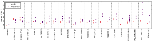
Figure 1. ECS estimated from recent (1979-2005) AMIP and historical simulations for each model’s ensemble of runs. Models are ordered by increasing estimated long-term ECS. Reproduced from Figure 1 of the Supporting Information for Marvel et al. (2018).
ECS estimates from historical simulations
The median ECS that Marvel et al. infer from1979-2005 historical simulation data is 2.3°C, significantly lower than the median long-term ECS estimate of 3.1°C.[12] However, there is an obvious possible explanation for these low ECS estimates from historical simulation data.
The 1979-2005 period is particularly unsuitable for ECS estimation since strong negative volcanic forcing arose during its first half, but not thereafter. There is evidence (including from Marvel et al.’s 2016 paper) that volcanic forcing has a low efficacy – it has much less effect on global temperature than the same CO2 forcing.2 [13] Accordingly, over the 1979-2005 period one would expect volcanism to increase the trend in F by a greater percentage than the trend in T, hence increasing the estimate of λ and depressing that of ECS.
It is simple enough to investigate the effect on short-period ECS estimation of avoiding significant influence from volcanism. I do so by using historical simulation data from the almost identical 1977-2005 period and Marvel et al.’s alternative decadal changes ECS estimation method. I made up the base ten years by combining the volcanic-free 1977-1981 and 1986-1990 periods. I took average changes from the base ten years to the final decade, 1996-2005, which is also free of eruptions. Doing so avoided the 1982 El Chichon and 1991 Mount Pinatubo eruptions and the main parts of the recoveries from each of them.
Figure 2 shows the resulting ECS estimates, upon applying equation (1).[14] The ECS estimates from individual simulation runs (red circles) are all over the place, as one would expect when estimating ECS from changes taking place over an average period of under twenty years. The change ΔF in average ERF is only 0.7 Wm−2, so in the odd run where a model exhibits large positive internal variability in ΔN between the split base period and 1996-2005 the denominator in (1) will be small, and thus the ECS estimate very high. In a modern observationally-based ECS estimate the ΔF value would typically be three times as large.
Where several historical simulation runs were carried out by a model, the ECS estimates using mean values from its ensemble of runs (red triangles) are less wild. But the interesting point shown in Figure 2 is that, across all models, the median of the long-term ECS estimates (blue line: 3.29°C) is almost identical to the median of the model-ensemble means based ECS estimates (red line: 3.37°C).[15] So, when care is take to avoid volcanism distorting the estimates, it is not true that ECS inferred from the recent historical period is “almost uniformly lower than that inferred from simulations subject to abrupt increases in CO2 radiative forcing”, as claimed by Marvel at el.
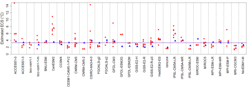
Figure 2. ECS estimated from non-volcanic periods in recent (1977-2005) historical simulations. Red triangles and circles show ECS estimated respectively from each model’s ensemble-mean values and from individual runs. Blue triangles show estimated long-term ECS. The red and blue lines (which overlap) show the multimodel-ensemble medians of respectively ensemble-mean ECS estimates and long-term ECS estimates. Long-term ECS was estimated using the same method as Marvel et al.
It is not possible to find a long period in historical simulations that avoids both significant volcanic activity and a large change in aerosol forcing. However, it is possible to improve the estimation of CMIP5 model ECS values by extending the period forward to 2016, splicing on data from RCP8.5 simulation runs that continue historical simulation runs after 2005, so as to use a final period of 2007-2016, as before taking changes relative to the combined 1977-81 and 1986-1990 periods.[16] The median within-model standard deviation of the resulting ECS estimates based on single simulation runs is then 13% of the median ensemble-mean ECS estimate. If that is taken as a proxy for the effect of internal variability on ECS estimation, it is not too bad given that this estimate is based only on data spanning a thirty year period, and on averaging over single decades.
For observationally-based energy-balance climate sensitivity estimation, where concern about model aerosol ERF strength is not a concern, one would normally use a much earlier (and typically rather longer) base period, thereby achieving a higher signal-to-noise ratio. If the full historical period to date is used to estimate model ECS values from simulation data, better precision is achievable. When using changes between the means for 1859-1882 and 1995-2016, two volcanism free periods, the median single-run ECS estimate standard deviation is only 8% of the median ensemble-mean ECS estimate. On that basis, uncertainty in observationally-based ECS estimation arising from internal variability is minor compared with other uncertainties.
ECS estimates from AMIP simulations
Marvel et al.’s median ECS estimate from CMIP5 AMIP simulations (1.8°C) was lower than that from historical simulations. A similar finding was shown (with volcanic years excluded) in Tim Andrews’ Ringberg talk in March 2015, and Gregory and Andrews (2016) gave sensitivity estimates for all models with AMIP simulations, albeit without identifying them, as well as their average.[17] It appears that the observed evolution of SST gave rise to enhanced tropical low-cloud cover compared to that in CMIP5 models’ historical simulations. The AMIP runs, which generally span 1979-2008, are too short to tell one much about the underlying cause, but in this case I think the lower ECS estimates for models are probably primarily genuine, rather than artefacts arising from use of a period with unbalanced volcanism. This is a reflection of Marvel et al.’s argument (c), which I put to one side earlier.
Marvel et al. claim that the low ECS values when models are driven by the observed evolution of SST patterns suggests that the “specific realization of internal variability experienced in recent decades provides an unusually low estimate of ECS.” However, as they admit, this is based on the perfect-model framework, which assumes “that the models as a group provide realistic descriptions of the mechanisms underlying observed climate variability“.
An alternative explanation for the models as a group misestimating the actual temporal evolution of SST change patterns is that the models as a group are imperfect. To my mind that should be the null hypothesis, rather than that internal variability over the last few decades results in an unusually low estimate of ECS. Indeed, the fact that internal variability linked to the Atlantic multidecadal oscillation is thought to have boosted warming over 1979-2005[18] makes it seem even less likely that in the real climate system ECS estimates based on this period would be biased low. Moreover, internal variability sufficient to produce a 20-year excursion of the magnitude required to account for the CMIP5 model average difference in N between AMIP and historical simulations does not appear to occurred in any of the 13,000 odd overlapping 20 year segments of their preindustrial control simulations.
Even if CMIP5 models don’t do too bad a job of simulating atmospheric behaviour, it is entirely possible that the real ocean is better able to move heat around the Earth’s climate system, in a way that reduces average surface temperature, than CMIP5 model oceans are able to do in their simulated climate systems. Marvel et al. recognize this, saying that the low ECS estimates derived from AMIP simulations “could also arise from the failure of the coupled models to reproduce aspects of the forced response”. Moreover, it is not the case that low model ECS estimates when driven by observed evolving SST patterns are limited to the last few decades. For now I will refrain from further discussion of this interesting area, which is a focus of current research activity, as this article is already overlong.
Endnotes and References
[1] The paper itself is pay-walled, but the Supporting Information is not.
[2] Marvel, K., Schmidt, G. A., Miller, R. L., & Nazarenko, L. S. (2016). Implications for climate sensitivity from the response to individual forcings. Nature Climate Change, 6(4), 386.
[3] They mention, as examples:
Gregory, J. M., R. J. Stouffer, S. C. B. Raper, P. A. Stott, and N. A. Rayner (2002), An Observationally Based Estimate of the Climate Sensitivity, J. Climate, 15 (22), 3117-3121;
Otto, A., F. E. Otto, O. Boucher, J. Church, G. Hegerl, P. M. Forster, N. P. Gillett, J. Gregory, G. C. Johnson, R. Knutti, et al. (2013), Energy budget constraints on climate response, Nature Geoscience, 6 (6), 415-416;
Lewis, N., and J. A. Curry (2015), The implications for climate sensitivity of AR5 forcing and heat uptake estimates, Climate Dynamics, 45, 1009-1023.
[4] In the outlier land use change forcing run by the GISS-E2-R model that they used, ocean convection appears to have partly collapsed in the North Atlantic, as it does in some of that model’s main CMIP5 simulations.
[5] Hansen, J. E. et al. Efficacy of climate forcings. J. Geophys. Res. 110, D18104 (2005).
[6] E. L. Davin, N. de Noblet-Ducoudre, and P. Friedlingstein (2007), Impact of land cover change on surface climate: Relevance of the radiative forcing concept. Geophys. Res Lett, 34, L13702.
[7] Armour, K. C., C. M. Bitz, and G. H. Roe (2013), Time-varying climate sensitivity from regional feedbacks, Journal of Climate, 26 (13), 4518-4534; Gregory, J. M., T. Andrews, and P. Good (2015), The inconstancy of the transient climate response parameter under increasing CO2, Philos. Trans. R. Soc. London. (Described by Marvel et al. as “in press” but in fact published in October 2015.)
[8] Byrne, B., and C. Goldblatt (2014): Radiative forcing at high concentrations of well‐mixed greenhouse gases. Geophys. Res. Lett., 41, 152–160, doi:10.1002/2013gl058456; and
Etminan, M., G. Myhre, E. J. Highwood, and K. P. Shine (2016): Radiative forcing of carbon dioxide, methane, and nitrous oxide: A significant revision of the methane radiative forcing. Geophys. Res. Lett. 43(24) doi:10.1002/2016GL071930.
[9] Since ECS is defined as the eventual temperature rise going from 1⤬ to 2⤬ (preindustrial) CO2 levels, and recent levels are approximately 1.4⤬ preindustrial. If feedbacks change with a perturbation of 4⤬ CO2, that would be a problem when using climate model simulations involving 4⤬ CO2 to estimate their ECS, as is typically done, but there is little model evidence of that being the case.
[10] See my analyses here and here. The best estimates of ECS for CMIP5 models are now generally obtained by scaling the x-intercept of a regression fit to years 21-150 of ΔT and ΔN data from a simulation in which a model’s CO2 concentration is abruptly quadrupled (‘abrupt4xCO2’), thus omitting the early decades in which higher feedback strength (lower sensitivity) is exhibited.
[11] They presumably estimated λ as the ratio of the inter-decade change in (ΔF− ΔN) to that in ΔT. This method is arguably more robust than using regression.
[12] Derived from scaling the x-intercept of a regression fit to years 1-150 of ΔT and ΔN simulation data after a model’s CO2 concentration is abruptly quadrupled. On average, this method appears to underestimate CMIP5 models’ ECS values, but only by 5-10% compared to estimates derived from the now generally preferred method of regressing over years 21-150.
[13] E.g., Gregory, J. M., Andrews, T., Good, P., Mauritsen, T., & Forster, P. M. (2016). Small global-mean cooling due to volcanic radiative forcing. Climate Dynamics, 47(12), 3979-3991.
[14] I derived ECS estimates for all models for which I could obtain data for their historical, preindustrial control and abrupt CO2 quadrupling experiments, using data from the latter two experiments to estimate a model’s long-term ECS.
[15] If 1977 and 1978 are excluded from the initial years, there is little change in the average ensemble-mean ECS estimate: the mean increases slightly and the median is marginally lower.
[16] I extended the AR5 forcing series from 2011 to 2016 using primarily observationally-based estimates. The resulting increase in anthropogenic ERF over that period was 0.23 Wm−2, the same as per the RCP8.5 forcings dataset.
[17] Gregory, J. M., and T. Andrews (2016), Variation in climate sensitivity and feedback parameters during the historical period, Geophys. Res. Lett, 43 (8), 3911-3920.
[18] E.g., DelSole, T., Tippett, M. K., & Shukla, J. (2011). A significant component of unforced multidecadal variability in the recent acceleration of global warming. Journal of Climate, 24(3), 909-926.

Reblogged this on Climate Collections.
They used model results, those are worthless, because the fundamental understanding of what’s really happening is being ignored.
Water vapor, because it is limited based on temp and pressure, regulates daily min temp. And you guys ignore this, because it actively changes the cooling rate at night, and that sets min T, and you can not have co2 warming without it impacting Min T.
Min T just follows dew point temp, and that follows the oceans.
https://micro6500blog.wordpress.com/2016/12/01/observational-evidence-for-a-nonlinear-night-time-cooling-mechanism/
Then if you use the extratropics know daily change in insolation, and compare that with the measured temp change at that specific station, that has a measured sensitivity of less that 0.002F/W/m^2
https://micro6500blog.wordpress.com/2016/05/18/measuring-surface-climate-sensitivity/
One of these years someone else will figure this out.
In one sentence: They confounded the low ERF of volcano forcing in the beginning of their considered very short time span (ElChichon 1982 and Pinatubo 1991) with a low ECS? This would be a “beginner mistake” and a regular peer review should have prevented this. It seems to me it was not as regular as it should have been:
” Publication History
Accepted manuscript online: 29 January 2018
Manuscript Accepted: 21 January 2018
Manuscript Revised: 18 January 2018
Manuscript Received: 27 November 2018″
Are you telling me even global warming alarmists now agree changes in atmospheric CO2 are not solely responsible for changes in surface temperatures due to their effects on radiative forcing? The monomaniacal fixation on magical properties ascribed to CO2 that are not seen in nature as the sole cause of global warming has been broken?
Executive summary: when the models conflict with the data, believe the models.
I had to laugh at this, because many years ago, a prominent paleoclimate modeler said this exact thing. He was talking to paleontologists, who had been perfecting their science for, oh,100 years or more. At the time, computer modeling of paleoclimate in deep time (i.e., before the last 2.5 million years) had been practiced maybe 10 years, if that. His talk was right after lunch, and everyone was dozing. I happened to be at the back of the room, and I never saw so many heads pop up in unison when he said that.
Thanks for deconstructing this new paper, Nic. Marvel has very low scientific credibility, and continues to demonstrate it.
Yes, unfortunately But look at the co-authors and the peers!
I think the main reason ECS estimates based on historical data underestimate the actual ECS is that the oceans are warming at only half the rate of the land due to their thermal inertia. The response so far has been disproportionately over the land compared to what the final response will be, likely underestimating the water vapor feedback which is delayed along with the ocean response to the forcing change. Just subtracting the imbalance in the denominator does not account for this delay in the water vapor feedback and is too simplistic for the real system that has multiple reservoirs with different heat capacities along the lines Armour has suggested. The warming of the tropical oceans is especially important to the water vapor feedback, and it has been slow so far compared to the global average.
JimD: Did you read the post or/and the paper?
I read the post. I can only see the abstract of the paper. However, my note is about why there would be an underestimate, regardless, so it gets at the main point of why this is expected anyway. It should not be surprising at all that models have a stronger long-term ECS for this reason.
100 years isn’t enough? How much longer is it going to take?
Jim D: Are you some kind of expert or just a blog person?
https://judithcurry.com/2018/01/16/sea-level-rise-acceleration-or-not-part-i-introduction/#comment-864600
yes
LOL
Lots of logical problems here:
I think the main reason ECS estimates based on historical data underestimate the actual ECS is that the oceans are warming at only half the rate of the land due to their thermal inertia.
You’re suggesting that response isn’t higher, because the oceans haven’t taken up as much heat as modeled (warming at half the rate).
Of course, most of recent papers make the opposite case: the oceans are taking up heat that would otherwise have shown up in the atmosphere.
Either way, it’s evidence that the models are in error.
Observed rates are at the low end of projections.
The IPCC AR4 made ‘projections’ in terms of the twenty first century.
The IPCC AR5, perhaps noting that warming was at the low end, went to the untestable ECS instead. This is troubling obfuscation.
The thirty year trend through 2017 is at 1.8C/century, the AR4 best estimate for a ‘low scenario’:
http://climatewatcher.webs.com/2017_NCDC30_TRENDS_COMPARISONS.png
TE, the oceans can take up heat and not warm as much. That’s what the high thermal inertia does. The heat is spread much deeper, and the surface cools less. Thermal inertia depends on both conductivity and heat capacity.
On ECS, if you look at the land trend (e.g. CRUTEM4), it is 0.3 C per decade. The land is able to keep up with the forcing better, and manifests the ECS magnitude better because it can adjust fast.
Higher ECS is possible.
But until there’s actually evidence to verify this, it is unsubstantiated speculation.
The land is already warming at a rate of 3 C per doubling, and this should not be ignored.
JimD: “…that the oceans are warming at only half the rate of the land due to their thermal inertia.”
This is not true! They are warming slower due to the limited WV in relation to the land. Try to learn some basics!
I meant: over land the (cooling) evaporation is limited, not so over the oceans.
Thermal inertia explains the diurnal cycle, seasonal cycle and climate change difference between the oceans and land. It is just harder to heat water, especially deep water, up than a land surface.
what are you talking about?
Thermal inertia does not explain the dinural cycle.
It self regulates due to the massive amount of water vapor, and the energy barrier of the state change as it’s cooled.
But I don’t expect you’ll understand it.
Nope.
Told you wouldn’t understand it.
I had no doubt about it.
You can tell it is not evaporation because in the seasonal cycle the land cools off faster in the winter too and that can’t be evaporation. It is thermal inertia.
It’s not from evaporation, it’s from as the days get longer more of the water vapor in the air gets condensed out. The air dries out, but there is still a barrier to cooling at dew point.
You can see this cooling and vacuum equipment, as they both get to a point where to go lower, it has to remove the water, and to do that you have to get rid of the extra energy stored as latent heat of evaporation, which is much higher than just reducing the temp.
That’s why the cooling rate at night changes from very fast at sunset, to even stopping cooling in the middle of the night.
All the while, it’s still bleeding energy.
JimD: The reason for the faster land warming under any forcing is well known since 1991, Manabe et al. It’s a “classic” paper : https://journals.ametsoc.org/doi/abs/10.1175/1520-0442%281991%29004%3C0785%3ATROACO%3E2.0.CO%3B2 Chapter 7 .
It is a well known lag, and the measured ocean warming rate is only half the land’s when you consider the last 30-40 years, so the point was that history-based ECS estimates ignore the delayed response in the water vapor feedback that goes with this. Such ECS estimates would be too low due to this.
It isn’t a delayed response, it responds differently.
This is part of the idiotic ideas ppl get when they pretend everything is a static average.
It’s a dynamic system folks! It responds in minutes!
JimD: repeating and repeating again the own assumptions vs. the results of the science makes no sense IMO. Did you read the linked paper Manabe et al. (1991)?
Frank, thanks for raising the Manabe paper to my attention.
I note:
“It is noted that the simulated response of sea surface temperature is very slow over the northern North Atlantic and the Circumpolar Ocean of the Southern Hemisphere where vertical mixing of water penetrates very deeply. However, in most of the Northern Hemisphere and low latitudes of the Southern Hemisphere, the distribution of the change in surface air temperature of the model at the time of doubling (or halving) of atmospheric carbon dioxide resembles the equilibrium response of an atmospheric-mixed layer ocean model to CO2 doubling (or halving). “
The ocean is warming at half the rate of the land.
http://woodfortrees.org/plot/crutem4vgl/mean:120/mean:240/plot/hadsst3gl/mean:120/mean:240/plot/crutem4vgl/from:1987/trend/plot/hadsst3gl/from:1987/trend
This has consequences for the water vapor feedback as I mentioned above. The ECS from such a non-equilibrium state of the climate would be deeply flawed if it ignored this factor, and the methods that just subtract the imbalance in the denominator do ignore it leading to a systematic underestimate of what happens when equilibrium is reached.
JimD: You made two mistakes: 1. You wrote “the ocean is warming at the half rate..” but you showed the SST. “The oceans” are not it’s surface!
2. The question was NOT : Are the SST warming slower? but: WHY? The answer to this question is given since 1991, see linked paper. The difference between TCR and ECS comes from the vertical heat distribution into deeper ( to about 300m depth) oceans. They have a much more bigger thermal inertia than the mixed layer depth which is the main contributor to the SST response. Due to the slow heating from GHG the thermal inertia of the slab ocean has no influence on the SST, it’s the saturated WV obove the water which leads to more evaporative cooling in contrast to the limited WV over land.
frankclimate, yes, it is the ocean surface which I plotted and is the temperature relevant to the response to forcing especially the water vapor feedback, and yes it is half the rate because of its effectively high thermal inertia due to deep layers having to warm. The first thing I wrote stands when you understand these things. This leads to a delay in the full feedback in response to warming which is the point. Evaporation is not the reason for the slow response, it is the thermal inertia. The Manabe makes no mention of evaporation for the reason that it is irrelevant, so I don’t know how you read that into it.
JimD. I don’t know how you can come to this conclusion ( thermal inertia) after reading my cited paper because Manabe didn’t mention this at all. Instead he writes: “Over the oceanic surface, saturation vapor pressure increases due to the surface temperature increase, thereby enhancing the evaporitive heat loss. On the other hand, the change in evaporation is smaller over continents where the rate of evaporation from the soil surface is less than the potential rate because soil is often not saturated with water. This land-sea difference in the CO2 iduced change of evaporative heat loss contributes to the land-sea contrast in warming…
Another relevant process is the positive feedback effect of snow cover….” ( Chapter 7 of this paper as I wrote before)
I retyped it for you because for this early pdf the coppy’n paste doesen’t work. Feel free to respond: “No, it’s thermal inertia!” In this case I can’t help you anymore.
It’s an interesting paper with a simplified ocean. If, as they say, the equilibrium warming pattern looks like the transient warming pattern, where does the fact that the ocean is warming at half the rate of the land take us? If this continues indefinitely, the land temperature continues to diverge and land takes up most of the global warming in the equilibrium state too. I somewhat doubt that these temperatures will continue to diverge at this rate. The current land warming rate easily exceeds 3 C per doubling.
http://woodfortrees.org/plot/crutem4vgl/mean:120/mean:240/plot/hadsst3gl/mean:120/mean:240/plot/crutem4vgl/from:1987/trend/plot/hadsst3gl/from:1987/trend
screen shots of Manabe 07, Role of Ocean Warming
https://i.imgur.com/WxyXjXH.png
https://i.imgur.com/dmAQY22.png
https://i.imgur.com/cYHNgCb.png
JimD: With this comment you admit that you didnt read this classic paper as you stated in this comment:”The Manabe makes no mention of evaporation for the reason that it is irrelevant, so I “. It’s a pitty that you are not a honest partner. I stop this conversation because it’s no use. Sorry.
I still don’t tend to go with single-paper conclusions, so you need more than that. If they predicted that the land would warm twice as much as the ocean, that would be interesting. If not, they are already wrong for some reason. I am open to the idea that the divergence could continue as it has for the last 40 years, but I suspect more that the ocean can catch up and close the gap once the forcing stops changing, and it is at that point that the assumption in history based ECS estimates breaks down.
What I find interesting in Table 1 is that the SH equilibrium response is larger than the NH, but the transient response is less. The transient response is consistent with it being mostly ocean, but the equilibrium response implies that the ocean does have to catch up given enough time. This is also not consistent with equilibrium and transient patterns being the same, so maybe that is not what they said.
Tim Palmer suggests here that greenhouse gases bias the climate system – and does a little experiment.
https://www.youtube.com/watch?v=w-IHJbzRVVU
Biases it to what? Abrupt and more or less extreme chaotic variability – of course. There is a theory that tectonic shifts changed a fundamental resonant frequency of the planet – and gave us 100,000 year glacials.
Hurst effects, tipping points, regime change, abrupt climate change – whatever you call it – are ubiquitous in the biological and physical environment of the Earth. A different sensitivity problem. Michael Ghil produced this energy balance model for his 1973 doctoral thesis – just a simple model of transitions in the climate system.
https://watertechbyrie.files.wordpress.com/2014/06/unstable-ebm-fig-2-jpg1.jpg
Solutions of an energy-balance model (EBM), showing the global-mean temperature (T) vs. the fractional change of insolation (μ) at the top of the atmosphere. (Source: Ghil, 2013)
The model has two stable states with two points of abrupt climate change – the latter at the transitions from the blue lines to the red from above and below. The two axes are normalized solar energy inputs μ (insolation) to the climate system and a global mean temperature. The current day energy input is μ = 1 with a global mean temperature of 287.7 degrees Kelvin. This is a relatively balmy 58.2 degrees Fahrenheit.
At transitions – that occur at all scales in the climate system – climate sensitivity is arbitrarily high. Between transitions greenhouse gases bias the system to transitions – I presume.
He does not agree with this:
https://i.imgur.com/6rJRjjh.png
I believe he might express it differently – but the bottom line is the same. Why don’t you ask? He is an approachable and agreeable enough fellow. Save me arguing more facile nonsense with an abusive climate change twit.
Here’s a picture from Slingo and Palmer 2011 that might help you frame some actually relevant questions.
https://watertechbyrie.files.wordpress.com/2017/04/slingo-and-palmer-e1506928933615.png
You have no memory. On CargoCult Etc., I am the person who originally linked to that diagram.
Prove it. Better yet – prove you understand what it means.
Lol. Right back at you.
Is the world warming?
“I would say undoubtedly that it is.” – Tim Palmer
Is it due to human emissions of CO2?
“I would say almost certainly it is.” – Tim Palmer
Will our continued emissions of CO2 lead to dangerous levels climate change (defined as greater than 2 ℃)?
“I will say it seems quite likely that will happen with any unmitigated emissions: continuing emissions.” – Tim Palmer
Stick to models – I am not going to indulge your shifting goal post fallacy.
“Indeed, the fact that internal variability linked to the Atlantic multidecadal oscillation is thought to have boosted warming over 1979-2005[18] makes it seem even less likely that in the real climate system ECS estimates based on this period would be biased low.”
Seeing that in the real climate system, AMO cooling in the 1970’s and mid 1980’s was ‘boosted’ by stronger solar wind conditions, and post 1995 AMO warming was ‘boosted’ by weaker solar wind conditions, ECS estimates must be biased way too high.
https://www.linkedin.com/pulse/association-between-sunspot-cycles-amo-ulric-lyons
“If it doesn’t fit, you must acquit.”
ATTP has been running a series of articles on ECS, including a discussion of Marvel on 30/1/2018 and one discussing the “one-box energy balance model” by Clive Best by Mark Richardson 1712018 and a new one by Andrew Dessler technically Dessler and Forster) 4/2/2018.
The gist of all the articles is that ECS is most likely 3.0 or higher with an inability or unwillingness to rule out much higher figures.
–
ATTP says “consider climate change specifically, then the no-feedback response is about 1.2K (i.e., the no-feedback response to doubling atmospheric CO2). This is largely because the Planck response is 3.2W/m^2/K and the change in forcing due to a doubling of atmospheric CO2 is 3.7W/m^2.”
–
This issue is very important as shown by the time and effort put into denigrating lower estimates like Nic and Judith’s.
The current trend is to blame the observations for showing lower climate sensitivity than the models and then using the models to prove it should be higher.
–
Basically a lot of the AGW concern falls over if ECS is 2.0 or less hence the concerted effort to deny this..
–
Andrew Dessler has an interesting take on using short term observations 2000 to 2017 to achieve an estimate that fits the models.
The only problem is a Gerghis like selectivity of the models he wishes to use for his Monte Carlo runs.
2, based on GISS, suggested ECS in the 1.0 or less range.
Fortunately these were not needed for the 15 out of 25 model ensemble used showing an ECS of average 3.3.
–
Nonetheless for ECS fans, good reading, and an excellent counterpoise to ideas here.
Yes. The GISS models are certainly outliers is various ways. But that doesn’t necessarily mean that what they imply about ECS is wrong. It has, incidentally, always struck me how different Gavin Schmidt’s views on ECS are with the behaviour of the GCMs developed at the GISS institute that he heads.
The biggest problem with Andrew Dessler’s approach is that, as he states in the paper, “the transfer function Θ_IV/ Θ_4xCO2 seems the most probable place for a significant error to occur” and they “have no way to observationally validate it, nor any theory to guide us”.
That transfer function is the scaling factor they use to converting observations of short-term, mainly unforced interannual climate variability to an estimate of the response of the climate system to long-term forced warming. It is the biggest contributor to uncertainty in their ECS estimate. They estimate the transfer function using GCMs, but if GCM’s high ECS values are mainly the result of their wrongly simulating long term cloud feedbacks then is is highly probable that their values for the transfer function will also be systematically wrong.
Thanks for clarifying where the problem may be.
The approach is still interesting and may lead to a way to narrow down the range if the model inputs are improved to enable a better match with the observations.
And it’s nonsensical. It’s less than 0.5C based on actual measurements of 2/3 the planet.
An additional 3.7W/m^2 to the surface at 288K with zero feedback gives 288.68K, and CO2 isn’t yet halfway to doubling from 280 ppm.
http://www.spectralcalc.com/blackbody_calculator/blackbody.php
I’d be careful here angech. ATTP doesn’t allow much diversity of opinion. He simply bans people who knowledgeably disagree. That makes his blog of limited value in terms of deciding or understanding things.
The real issue here (and one that Dessler, ATTP, Marvel, and the whole crew ignore) is the series of recent papers with negative results about AOGCM’s and indeed AGCM’s. I’ve tried to get some response to this and there is never any response. That’s a classical public relations stunt. Ignore any evidence you don’t like and just repeat your opinion or lines of evidence you do like.
Nic’s recent writeup on ECS is really excellent on this point however and gives a whole list of references.
actually Dressler himself answered the questions
dpy6629
One gets value out of blogs in many ways. The old Sherlock Holmes thing. The things that get banned for instance might suggest the ideas that bite the hardest.
So sometimes what is not said at a blog is even more interesting than what is being said.
Ignoring papers with negative results is one thing, Reacting to papers with opposing conclusions is another.
Here we have a whole series of wars going on about several topics.
Low ECS is one.
It is the garlic and holy water, the silver bullet and wooden stake to the notion of AGW.
How can AGW be important if ECS is low. AGW would die as a problem.
Hence the response.
Denigrate the opposition – they are not scientists .
Ignore.
When they are scientists – denigrate the person to denigrate the research.
Publish articles proving – ECS is high – the skeptic research was wrong – or the scientists were not real scientists as they are not accepted in the scientific community.
–
Here we have the second approach, an avalanche of articles tying themselves in knots, trying to prove an unprovable.
Why unprovable?
Simply because the observations do not agree with the theory and are currently diverging rapidly wh the El Niño subsidence.
The explanations all differ and become more and more bizarre.
I see numbers of otherwise sensible scientific bloggers making irrational statements.
Deciding post experiment on which results to include and which ones to discard.
Sad.
But it also means they are losing this argument badly
Hence the response.
You just can’t stop yourself. You are completely wrong.
Mosher, What was Dessler’s alleged answer? If he answered my question, I missed it.
one place
> it also means they are losing this argument badly
This impression of yours may only be reinforced by the conclusion that contrarians always win, Doc:
https://andthentheresphysics.wordpress.com/2018/01/11/can-contrarians-lose/
In any case, have you noticed how you’re being told that you’ve not banned because you’re not knowledgeable or something?
Please don’t tell that to CliveB or NicL.
> it also means they are losing this argument badly
I can’t imagine where this comes from, but sober up dude, they’re winning it in a runaway. Observations are going to keep rocking upward unless you get a string of fairly powerful La Niña events, and that is not, so far, happening.
PDO back up; La Niña pooped out:
https://i.imgur.com/iHBVUS0.png
https://i.imgur.com/x6jCgyR.png
https://i.imgur.com/AzsW7B8.png
JCH: elsewhere you made some comments about AMO and “fibbers”. If you find a way to read this paper: https://journals.ametsoc.org/doi/abs/10.1175/JCLI-D-17-0444.1
… do so!
That’s a non response response JCH. Basically we share your frustration with AGCM deficiencies but the relationship we are looking at is well modeled. Didn’t see any evidence cited. Tropical convection will affect their relationship I would argue. That’s a particularly weak area for GCMs
Is the AMOC the same as the AMO?
“Is the AMOC the same as the AMO?”
Don’t lower the bars too much!
http://www.ospo.noaa.gov/data/sst/anomaly/2018/anomnight.2.5.2018.gif
So much blue seems apropos that Bobby Viinton would reprise his hit.
JCH “> it also means they are losing this argument badly” , I can’t imagine where this comes from”
I guess I am the one needing a reality check?
–
“Observations are going to keep rocking upward unless you get a string of fairly powerful La Niña events, and that is not, so far, happening.”
–
So, you are asserting that you know for sure when the nex El Niño and La Nina’s are going to come and how big they are going to be?
I don’t think so either.
Hence, like everyone else you have no knowledge if observations are going to keep rocking up, no information on when the next string of fairly powerful La Niña events will occur ( they will occur that much we know) but use your gut feeling combined with the science of CO2 increase to make a prediction that feeds your idea of the future.
–
For the record a string of fairly powerful La Niña events could start right now.
If they did we would certainly not see observations rocking up.
Likelihood ?
Probably 2-5% right now. Or at any time really, the truth is you will not know it is happening til it is well underway but it could be happening right now.
“PDO back up; La Niña pooped out:”
According to your graph we need February below -0.5 and we are back in the blue 5 month new La Niña, that cannot be right??
The La Niña simply has not latched. Warm surface waters keep appearing along the equator. So it is already starting to end. Will it make 5 periods? Yes, but it is going to be weak. Face it now; face it later; I don’t care.
Through 2017:
https://i.imgur.com/Ks2UTU8.png
OHC:
https://i.imgur.com/clyJW3y.png
Observations. All of them going against you.
And, we’re in a string of La Niña events: two in a row. That’s whit has been so chilly: 4-alarm chilly. How likely is a 3rd in a row?
And, we’re in a string of La Niña events: two in a row. How likely is a 3rd in a row?
Even money.
El Niño and La Niña episodes typically last nine to 12 months, but some prolonged events may last for years. While their frequency can be quite irregular, El Niño and La Niña events occur on average every two to seven years.
–
Let’s say next event in 4 years.
So 50 % chance of three in a row in just the next 4 years, possibly in 2 years if it comes early.
–
Plus you did not mention the lag time for temperatures to follow events nor the almost El Niño at the start of 2017.
You should not be scared to talk about and acknowledge such things for fear of upsetting your argument. You would get greater respect, well from the skeptical and scientific communities if you did.
–
Your stated position this year is still 2018 as top 5?
You have a good base to start from but due to your intransigence in respecting the lag I think your prediction will struggle to make first 5.
11 months to go.
Thank you for your timely warning David.
I hoped it was not right and even had a little angst when one of ATTP’s regulars took me to task for not “straightening the record”
Alas you were right .
ATTP put up a post ” A challenge for my readers””
Posted on February 11, 2018 Topic
John Cook and colleagues have new paper out about [d]econstructing climate misinformation to identify reasoning errors.
–
I made some constructive comments and Mosher put out a challenge to challenge just one of the errors and misstatements.
I did so in this comment
At last a real discussion Posted on February 15, 2018 by angech
–
I am appreciative of your pointing out some of the difficulties in giving cogent arguments to every problem when some appear to have been rushed or not explained as well as they could be.
Came across an Aussie? Steve Sherwood Director, Climate Change Research Centre, UNSW with a piece showing the problems with using the hot spot argument. “” Climate meme debunked as the ‘tropospheric hot spot’ is found ” ** 2015
1. If you cannot find it, debunk its importance by saying it is a general sign of temperature increase, not a fingerprint of climate change.
2. If you can find it, insist on its importance as proof.
This article happily does both.
–
Quoting Skeptical science [abridged by me]
“Why should there be a ‘hotspot’ in the atmosphere above the tropics?
Most of Earth’s incoming energy from the sun is received in the tropics, strong evaporation there removes a lot of heat from the ocean surface. This heat is hidden (latent)
Strong evaporative uplift occurs near the equator due to the intense solar heating of the ocean there, forcing s the evaporated water (water vapour) to ascend up through the atmosphere. Because the temperature in the atmosphere decreases with increasing height (known as the lapse rate), this has the effect of cooling water vapor until it reaches a point where it condenses back into a liquid form (forming clouds and rainfall) – liberating the hidden (latent) heat into the upper atmosphere. With the great bulk of atmospheric moisture being concentrated in the tropics, this ongoing process should lead to greater warming in the tropical troposphere than at the surface.”
–
The problem
“Despite obvious warming of the atmosphere, it had been difficult to confirm the existence of this hotspot *” Skeptical science
The talking point?
The answer is not that any cause of temperature rise should give a hot spot.But that a temperature rise seems to have occurred but the warming spot has not.This then allows for doubt to be cast unfortunately on the measurements of temperature.
Which opens the whole can of worms,
[” Show one “skeptic” point to be correct, and then show how that point being correct “adjudges” all “skeptic” arguments (or even a lot of them, or even one of them). “]
–
*primarily due to analytical deficiencies in accounting for temperature data quality and sampling, i.e. it’s suspected to have been a ‘measurement problem’. Skeptical science
**”The problem is that temperatures vary during the day, and when a new satellite is launched (which happens every few years), it observes the Earth at an earlier time of day than the old one (since after launch, each satellite orbit begins to decay toward later times of day).” Sherwood
–
Which sadly did not see the light of day.
Seems ATTP doesn’t allow much diversity of opinion. He simply bans people who knowledgeably disagree..
I make this posting to let Mosher know I did reply and to raise awareness of the difficulty in communicating with people with fixed mind sets.
Who pretend to be willing to have a discussion and then delete comments and run.
The greatest feedback, as understood by Soden and Held 2006, is the positive water vapor feedback.
To get high ECS, the atmosphere needs WV feedback.
And to get WV feedback, the atmosphere need the Hot Spot.
With every passing year, the Hot Spot becomes more and more conspicuous by its absence.
The biggest feedback is negative – the Planck response.
The Hot Spot would also be part of the negative lapse rate feedback. It’s absence only makes it worse than we thought.
On the other hand – an absence implies less atmospheric warming.
No, it implies the full water vapor feedback hasn’t kicked in yet at least in those regions.
The ‘hot spot’ results form atmospheric warming – for any reason. It is not strictly about more water vapor – just where it cools. Although a warmer atmosphere and water vapor seem to go hand in hand.
The warmer atmosphere goes with more water vapor because of the feedback, but sometimes that part is delayed, hence a weaker hot spot. But the hot spot is connected to more water vapor, and would not occur unless there was.
No, it implies the full water vapor feedback hasn’t kicked in yet at least in those regions.
Unfortunately for your thesis, there is observational evidence that water vapor feedback hasn’t kicked in. There is no observational evidence that water vapor will ever kick in.
It’s still a free country. You can speculate all you want. But verification is still a matter of observation.
Actually it kicks in every clear night, it’s just an anti-co2 forcing change feedback.
https://i1.wp.com/micro6500blog.files.wordpress.com/2016/12/1997-daily-cooling-sample-zoom-with-inset1.png
The Hot Spot would also be part of the negative lapse rate feedback. It’s absence only makes it worse than we thought.
The absolute value of the water vapor feedback is larger than the absolute value of the opposing lapse rate feedback.
So the absence of the hot spot means less temperature feedback, which is consistent with the low observed temperature response.
Also, “worse than we thought” is a fingerprint of bias.
TE,
thanks for keeping trying to nudge the conversation back to science and objective observations.
Scott
The sensitivity is well ahead of the no-feedback 1 C per doubling, just from observations (1 C already with half a doubling), and only the added global water vapor, which has been measured, can account for the extra warming. So, yes, water vapor is increasing and helps explain the doubled effect. Moisture laden areas like the tropical oceans will warm less quickly because the CO2 effect is more masked at the surface there.
No the problem is still quite bad with an ECS of 2.
given the difficulty of changing our energy consumption.
You need an ECS of less than 1 with CERTAINTY to have a worry free future.
Anything 2C or over is reason for concern and some measure of repsonsible action towards mitigation
“Anything 2C or over is reason for concern and some measure of repsonsible action towards mitigation”
You called the right number. The Party Line.
Andrew
We have measurements of sensitivity to insolalation for 2/3rd the planet.
https://micro6500blog.wordpress.com/2016/05/18/measuring-surface-climate-sensitivity/
While the graphs are Watt Hr(Work)/m^2/Day, the highest point at the beginning of the records from Antarctica based on only a few stations, most the rest the planet is half that peak rate (0.02F/Whr/m^2/Day, or 0.0004C/W/m^2/day)
“Anything 2C or over is reason for concern and some measure of repsonsible action towards mitigation”
The switch to natural gas was “some measure of responsible action.” Can we all clap and go about our business now? Or do you still want to power California with windmills by the next presidential election at any cost or reliability?
The transition to electric cars and nuclear power over the next 3-4 decades will be both natural and inevitable (depending on battery tech). Is that fine or does Bill McKibben need to stand in front of bulldozers this year as he wrote in the Guardian recently?
So much wiggle room in “some responsible action”. But then that’s been the whole debate since ’88 where one side says it means ending democracy and capitalism and the other notes that technological innovation solves the problem (such as figuring out how to make natural gas supplies so prevalent and cheap that we start replacing coal with it because it makes economic sense.)
A question- it’s been 30 years since James Hansen told the US Congress a projection of warming that’s now recognized as ludicrously high, the projections keep dropping and billions of dollars in spending haven’t made renewables any more attractive or likely. Who do you think deserves the first apology?
Steve Mosher,
There is a missing step in there: you also need convincing evidence that 2C ECS presents serious problems. (By serious problems I mean problems which will be difficult to address via technology and adaptation.)
A meaningful policy discussion needs to honestly address projection of future CO2 emissions absent any mitigation efforts (and that is not the scare-story 8.5 scenario), honestly address the likely temperature response, as well as the likely consequences of that temperature response. So long as one side in the discussion insists on basing policy on wildly unrealistic emissions scenarios, worst case temperature response, improbable consequences (1.5 meter sea level increase in 80 years! Miami disappears! Many places become uninhabitable by humans!), while simultaneously ignoring both the economic/social costs of mitigation policies and the long term contribution of technology in solving problems, meaningful policy discussions are essentially impossible. The endless caterwalling of alarm tropes only serves to delay a serious policy discussion.
Steven, albeit I mostly agree with you here I tend to disagree. The question was NOT how mankind should react to ECS>1, the question was: are the conclusions of Marvel et al ( ECS>>2) bolstered by the methods in this paper. And IMO this is not the case as Nic showed. One should seperate: here Nic discussed the science, not if we have to worry about the future. This is not the business of the scientific community but for politics. I know that in almost every case in response to any special study the commenters come to the basic physics ( greenhous effect ect.) which is a pitty and lowers the bar of the discussions here IMO. .
Anything less than 1 is reason for concern, you need 2 or more to have a worry free future. For those who believe or live off the scare.
> albeit I mostly agree with you here I tend to disagree.
Mostly.
“The switch to natural gas was “some measure of responsible action.” Can we all clap and go about our business now? Or do you still want to power California with windmills by the next presidential election at any cost or reliability?”
As a supporter of fracking I agree.
I have no idea how I want to power California.
Ideally I’d leave it to californians to decide.
They have lots of valuable coast line and are best positioned to
decide.
HOWEVER, there future is also in my hands and in the hands of
India and China.
Its a tough question.
I wont be around to face the consequences of offering the wrong
advice. So I am circumspect.
“The transition to electric cars and nuclear power over the next 3-4 decades will be both natural and inevitable (depending on battery tech). Is that fine or does Bill McKibben need to stand in front of bulldozers this year as he wrote in the Guardian recently?”
Do I look like Bill McKibben? FFS. I answer for me, you clown.
I do not answer for Him, take questions for him, or feel any
responsibility to explain, defend, accept or reject his ideas.
Am I Bill? really? did you mistake me for him?
“So much wiggle room in “some responsible action”. But then that’s been the whole debate since ’88 where one side says it means ending democracy and capitalism and the other notes that technological innovation solves the problem (such as figuring out how to make natural gas supplies so prevalent and cheap that we start replacing coal with it because it makes economic sense.)”
HUH? you dolt, why are you lecturing me of all people about natural
gas? And innovation? you really are clueless about my positions.
There is no clear optimal answer to the concern. We have three
tools: Mitigation: Adaptation: Innovation. In the end we may need
all 3. How much of each? Totally unclear and not my decision.
A question- it’s been 30 years since James Hansen told the US Congress a projection of warming that’s now recognized as ludicrously high, the projections keep dropping and billions of dollars in spending haven’t made renewables any more attractive or likely. Who do you think deserves the first apology?
Hansen was not wrong. His prediction was pretty darn good considering all the uncertainties. If you had ever spent a day working
in Highly uncertain projections you’d see his projections as a huge
success. wrong of course, but thats a given
frank
angech claimed
‘Basically a lot of the AGW concern falls over if ECS is 2.0 or less hence the concerted effort to deny this..”
I’m responding to that.
Thanks for almost agreeing with me
“clown”
“dolt”
Stay Classy!
“Hansen was not wrong.”
Hansen told Congress in 1988 that ECS was 4.2. He was not wrong in the same sense that The Population Bomb (millions dying of starvation in the US in the 1980s) was “not wrong.” If you propose to have politicians base policy on this sort of thing, this matters.
“There is no clear optimal answer to the concern. We have three
tools: Mitigation: Adaptation: Innovation. In the end we may need
all 3.”
And the choice, policy-wise, is determined by the seriousness of the threat. Hansen’s projection would be akin to telling New York to evacuate ahead of tomorrow’s hurricane (and calling it “not wrong” if there is a bit of rain tomorrow. ) Do you not grasp how projections impact policy, or do you not recall the last three decades of hysterics?
Hansen, for example, said it was suicide to develop natural gas. People who suggested it as a “responsible” action were derided as “clown,” “dolt” and it was even suggested they be arrested.
You have no responsibility to call out McKibben but you think Curry has a responsibility to call out sky dragons. Bill McKibben is now a “denier” and has the ear of one entire US political party, it seems pretty obvious to me that anyone who is serious (key word) about climate change has an interest in responding to him.
“I have no idea how I want to power California.
Ideally I’d leave it to californians to decide.
Do Indianans get this choice too or only states that propose the ridiculous? FFS, based on an exaggerated estimate of global warming we’ve wasted a third of a century letting the politicized lecture us that only the most wildly unlikely mitigation policies are acceptable – a tactic so poisonous that to this day it means climate science prioritizes bad estimates for the sole purpose of pushing unjustifiable policy choices. If you care about climate change you need to care about how California is powered because they will be either a good or bad example.
Steven Mosher
“No the problem is still quite bad with an ECS of 2.
You need an ECS of less than 1 with CERTAINTY to have a worry free future.Anything 2C or over is reason for concern and some measure of repsonsible action towards mitigation”
Given that ECS for doubling is > 1.0 without feedbacks you seem to be saying that the system we live in is a failure and poorly designed.
Amazing that life has been able to survive and adapt through so many past multiple doublings and droppings.
Perhaps we can put a carbon tab on Vulcan and Gaea for their thoughtless behaviour and failure to turn the lights off.
–
I worry about a future without readily available power. I worry about the people in the world without power now.
Real people.
Hurting real people now is actual damage.
Hurting people who may never exist is a mind game.
One is a criminal activity, an act of commission.
The other is a thought process, a bubble of omission.
To civilised people there is a yawning gap.
“There is also a puzzling peak below 1°C. These low values come from the GISS models (Fig. 7a) and if they are removed from the ensemble, the bump below 1K disappears .
We find that 15 of the 25 CMIP5 models produce estimates in agreement with the CERES
observations. If we limit the distributions to just those models , we obtain the ECS distribution in Fig. 6c (hereafter referred to as the “good” distribution).
We consider the “good ” ECS distributions to be the best estimates of ECS from this analysis.
Those ECS distributions have 17-83% confidence intervals (corresponding to the IPCC’s
likely range) of 2.4-4.4 K ”
You chopped a bit of text, Doc:
https://andthentheresphysics.wordpress.com/2018/02/04/ecs-from-a-modified-energy-balance-approach/#comment-111219
Care to try again?
Words.
I did not drop a bit of text, I summated a lot of text into the appropriate, short, take home messages. I did not leave out conflicting explanatory, agreeing or disagreeing bits accidentally. I took the bulletproof points and put them together leaving the verbiage out.
Legally, ethically and morally I feel comfortable with this approach. I would hope that I am moral enough to put up a valid counterpoint if one is presented at the same time. Remember, these are his words, not mine and people are free to look up the context if they wish.
I will happily put up retractions if you can point out where I have made a deliberate misquote or manufactured a meaning not there.
Nothing you have quoted disproves or alters those points in any significant way.
Andrew did qualify and explain his comments and I have no problems with the fact that he did do.
> leaving the verbiage out.
You mean, like the words that answer the rhetorical question you asked at AT’s, perhaps?
That’s some weird way to pay due diligence to the concerns AndrewD had to spell out for you, Doc.
No,
“Andrew did qualify and explain his comments and I have no problems with the fact that he did do.”
In terms of the bullet points made the extra comments were redundant, not germane, of no extra value to the concept and argument made.
You can fight as long and hard as you like, shift the sands of the argument and pretend that you do not clearly understand what I am saying.
The argument is not misquoting or dropped bits of text though it appears you would like it to be in the absence of any real discussion that you said
you would like to have.
Argue on the relevant points, or choose to distract, I do not mind too much.
People read the statements.
They can choose which ones have character, belief and resonance.
So go for it. Keep digging.
Andrew Dressler has put a good idea out for a shortcut in ECS estimation
Nic Lewis says it is hard to do with all the confounding factors.
Yet both of them are trying and to be congratulated.
The fact that GISS observations fail to fit his theory is not a problem.
He does not see it as a problem.
It is a way to get an improvement next time.
He and Nic, could work on it ( they won’t I guess) and get an amended version with a lower ECS up.
If not, the truth will out in time with observations, not models as the proof of the pudding.
> In terms of the bullet points made the extra comments were redundant, not germane, of no extra value to the concept and argument made.
The very first sentence you chopped, i.e.:
refutes your claim, Doc. It also answers in part your rhetorical question, by offering a reason why removing the low values makes quite a bit of sense.
***
> You can fight as long and hard as you like, shift the sands of the argument and pretend that you do not clearly understand what I am saying.
You need to say it first, Doc.
Since you’re acting tough all of a sudden, why don’t you spell it out for once?
Willard
“It also answers in part your rhetorical question,”
A rhetorical question by definition answers itself, doesn’t it?
Hence
“offering a reason why removing the low values makes quite a bit of sense.”
Implies it was not a rhetorical question.
–
“Since you’re acting tough all of a sudden, why don’t you spell it out for once?”
Sorry, I am not getting into a cage fighting scenario with a seasoned cage fighter, give me some sense.
–
“There is also a puzzling peak below 1°C. The only way for an ECS estimate to be close to zero is if Q iv is very large or one of the other terms in Eq. 6 is close to zero. Analysis of the terms in Eq. 6 suggests that the term causing the low ECS values is Q iv /Q 4xCO2 , whose distribution approaches zero (Fig. 4a). These low values come from the GISS models (Fig. 7a) and if they are removed from the ensemble, the bump below 1 K disappears (Fig. 6b)”
–
Translation(s)
Our method shows that the scaling factor Q iv /Q 4xCO2 is unconstrained by (does not work with all) observations.
Since 4xCO2 is invariant the problem has to be in the other observations.
Two GISS models give a result showing negative feedbacks.
Since negative feedbacks < 1.0 are forbidden as they will stop Mosher from worrying we will remove them and only follow the models which fit what we predict.
The rhetorical question was that though this method works and may well be right is it a correct and rigorous approach?
Should more work be done on finding why the anomalous and seeming in error results came about?
> A rhetorical question by definition answers itself, doesn’t it?
Depends. There are many types of rhetorical questions – e.g. your “doesn’t it” is a suggestive question. Sometimes, what’s being intimated is more or less obvious, like in the rhetorical question we’re discussing:
I contend that you may have a hard time spelling out your concern. Not that it matters much when dogwhistling.
See? That last rhetorical question didn’t answer itself either!
***
> Since negative feedbacks < 1.0 are forbidden as they will stop Mosher from worrying
You might not be justified in putting these thoughts into Moshpit's mouth:
https://judithcurry.com/2018/02/05/marvel-et-al-s-new-paper-on-estimating-climate-sensitivity-from-observations/#comment-865693
Considering that an ECS of 1 or less is barely physical, I’d be more worried about our scientific understanding than Moshpit’s mind.
***
> I am not getting into a cage fighting scenario with a seasoned cage fighter, give me some sense.
Then maybe you shouldn’t talk in people’s back, should you?
Pingback: ecs 2018 | asoliduniverse
Can’t understand why we obsess with scary ECS estimates when we are about to find out.
Why this focus on ECS?
The concept of equilibrium CO2 levels is at odds with the peak oil scare and limits to growth. You can’t bave both, so what is it?
We are observing a constant airbirne fraction of CO2 which disproofs the dreaded sink saturation of the Bern model.
The necessary components for Catastrophic Anthropogenic Grobal Warming (CAGW) are:
1 An over the top emission scenario like RCP8.5;
2 Sink saturation which keeps this CO2 in the atmosphere;
3 A high value for climate sensitivity.
I would call this a science fiction horror scenario, not science, because all three components are highly unlikely.
Finally climate sensitivity has a very strong frequency component so climate models should study a pulse response of CO2 which is far more like the peak oil concept. Ramp and equilibruim forcing of climate models yield over the top TCR and ECS values which have no meaning in a pulse like CO2 emission.
This low amplifier spectrum gives a more realistic picture of the frequency responce for climate sensitivity, (note the resonance peaks!)
https://www.innerfidelity.com/images/shure_se535_graph_comparison.jpg
See also the paper
The Frequency Response of Temperature and Precipitation in a Climate Model by Douglas G. MacMynowski,, Ho-Jeong Shin and Ken Caldeira
on the concept of frequency domain climate sensitivity
http://www.cds.caltech.edu/~macmardg/pubs/SP_GRLfrmt.pdf
Reblogged this on I Didn't Ask To Be a Blog.
” current climate models show a lower sensitivity when their atmospheric modules are driven by the observed historical evolution of sea surface temperature (SST) patterns;”
Interesting in this regard the recent Severinghaus (2018) noble gas measurements suggesting ocean warming over the last 50 years of only .1C.
“Where precision is an issue (e.g., in a climate forecast), only simulation ensembles made across systematically designed model families allow an estimate of the level of relevant irreducible imprecision.” James C. McWilliams
At the core of models are Navier-Stokes equations in 3 dimensions. They are solved numerically and preserve momentum across grid boundaries.
https://upload.wikimedia.org/wikipedia/commons/b/b1/Global_Climate_Model.png
The equations are nonlinear and generate divergent solutions from small initial differences. In a practical sense – initial differences far greater than Jimmy D’s ten to the minus fourteen Kelvin.
Model solutions in the CMIP are not model solutions but one realization of a control run projected forward in time. There are no unique, deterministic solutions. They are model runs from a specific starting point that exist within an envelope of model uncertainty – the fractionally dimensioned solution space of “systematically designed model families”. There is no rigorous justification for any of the choices in CMIP. Merely mirrors of the bias of modelers. The ‘solutions’ are about as useful for determining sensitivity as a bicycle is for a fish.
So I never understand any of this endless quibbling about angels from pinheads.
The differences grow to a degree in the first few months. Isn’t that enough of a perturbation for you? This is Lorenz-type growth relevant to the deterministic predictability range.
http://www.cesm.ucar.edu/projects/community-projects/LENS/images/Figure2.gif
I don’t know what this is meant to mean. My guess would be not much.
Yes, maybe you don’t know that the size of the initial perturbation is immaterial after a few months. See Lorenz.
What I do know is that you talk absolute nonsense. See Lorenz? Nuts.
Clearly you need to understand what Lorenz has said about the butterfly effect. Let me help. Small perturbations grow and saturate the variance after only a few weeks. That’s what limits predictability.
Clearly you have demonstrated that you have not the slightest clue. And this is just one more instance.
Lorenz: “Two states differing by imperceptible amounts may eventually evolve into two considerably different states … If, then, there is any error whatever in observing the present state—and in any real system such errors seem inevitable—an acceptable prediction of an instantaneous state in the distant future may well be impossible….In view of the inevitable inaccuracy and incompleteness of weather observations, precise very-long-range forecasting would seem to be nonexistent.”
Yes we clearly understand what sensitive dependence on initial conditions is.
What you have added is that the quantum of initial differences is immaterial and that divergence ceases after weeks to months. This latter is made up nonsense.
When do you think the divergence ceases if you look at the LENS results? In a short time the variability among ensemble members is at a maximum, well within the first year which is 1920. Lorenz has put the growth at a few weeks, but you don’t, so say how much you disagree with Lorenz.
http://www.cesm.ucar.edu/projects/community-projects/LENS/images/Figure1.gif
Not the case. There used to be a single weather forecast that diverged from weather after about a week. These days the emphasis is on probabilistic forecasts.
The LENS modelling you refer to uses a single control run projected forward. There are many other solution trajectories possible starting from realistic values of input parameters and that diverge through to the end of the century at least. The experiment has been done.
Your results use minuscule initial differences – 1E-14K – to limit uncertainty around that non-unique trajectory to a 0.4K range supposed to mimic natural variability. It doesn’t – climate will diverge from models just as weather does and may be more or less extreme. Nor do they model the physics of natural variability – merely mimic expectations through sensitive dependence and minute initial differences diverging around a single chaotic trajectory.
There are 1000’s of other realistic trajectories possible – each with the potential for minute perturbations to cause variability around it of 0.4K. Or even much more with larger – more realistic – parameter variations.
Climate will continue to diverge from models and probabilistic – hardly deterministic – climate forecasts when they happen some time or other are the best that can contemplated.
It has been shown conclusively that your repetitive peregrinations of this is utter rubbish. We cannot hope that anything at all will cause you to rethink any of your ad hoc rationalizations. It is by no means uncommon – but you are stuck in a meme warp.
“Simplistically, despite the opportunistic assemblage of the various AOS model ensembles, we can view the spreads in their results as upper bounds on their irreducible imprecision. Optimistically, we might think this upper bound is a substantial overestimate because AOS models are evolving and improving. Pessimistically, we can worry that the ensembles contain insufficient samples of possible plausible models, so the spreads may underestimate the true level of irreducible imprecision (cf., ref. 23). Realistically, we do not yet know how to make this assessment with confidence.” James C. McWilliams – http://www.pnas.org/content/104/21/8709.full
So, in all that you haven’t said why the LENS results don’t diverge beyond half a degree for the 180 years that they are run. Again, see Lorenz. There is an attractor and that limits the range of temperature excursions from the mean. The same happens with weather in nature as suggested by Lorenz. As McWilliams says, you need ensembles, but even they have their limits.
You imagine that the attractor is something strange. What McWilliams says is you need ‘systematically designed model families’ to determine the limits of a model uncertainty. If you read any of the contemporaries cited – you might understand. As it is – I don’t really know what to make of your meme warped arguments.
We have on the one hand minute – 1E-14K – pertubations that result in one solution space – or strange attractor as you seem to have newly discovered – intended to produce 0.4k uncertainty – and on the other plausible physical parameters that produce a much larger solution space.
Lorenz I can inform you has never insisted that the dimensions of the strange attractor was invariate in all cases. That seems to be what you are saying – although it is far from obvious that you say anything much at all of interest.
You seem to think that a chaotic system still remembers the size of the initial perturbation after 180 years. Lorenz would say any memory of it disappears in a few weeks in the case of weather systems. If the figurative butterfly flap can grow into a hurricane in a few weeks, think what that hurricane can do to the later forecasts with the butterfly long forgotten.
No – just that the initial difference is so much larger. This is not something that is speculative – the subject of specious physical reasoning seen all too often. Cyclones for instance. It is a computer program – something that can and has been run many 1000’s of times. There are results that have been discussed endlessly with you. The way to reduce ‘the fractionally dimensioned space occupied by the trajectories of the solutions of these nonlinear equations’ is to improve observations and reduce grid size.
The difference grows exponentially and then saturates at weather-scale differences that you would get by comparing random days. So after only a few weeks the difference between members is as large as it can get. Why do you not think that can be true? Annual differences of 0.5 K are what is expected and those annual variations are seen in the global mean observations too.
No – just that the initial difference is so much larger. This is not something that is speculative – the subject of specious physical reasoning seen all too often. Cyclones for instance. It is a computer program – something that can and has been run many 1000’s of times. There are results that have been discussed endlessly with you. The way to reduce ‘the fractionally dimensioned space occupied by the trajectories of the solutions of these nonlinear equations’ is to improve observations and reduce grid size. Even then – as I keep quoting – “we should expect a degree of irreducible imprecision in quantitative correspondences with nature, even with plausibly formulated models and careful calibration (tuning) to several empirical measures.”
I agree with McWilliams, as I have said. There is a limit to predictability of something like a monthly average temperature, or even annual average. He’s talking about prediction. You can predict an annual average to within 0.5 K, however, because that is the variation range. Frank’s random walk model doesn’t even allow that level of precision to be possible, right?
I have read the McWilliams paper many times now – I don’t think I get what you get.
“Sensitive dependence and structural instability are humbling twin properties for chaotic dynamical systems, indicating limits about which kinds of questions are theoretically answerable. They echo other famous limitations on scientist’s expectations, namely the undecidability of some propositions within axiomatic mathematical systems (Gödel’s theorem) and the uncomputability of some algorithms due to excessive size of the calculation.”
McWilliams says that the atmosphere-ocean system is perhaps more chaotic than the atmosphere alone, but experiments like LENS had not been done yet. LENS results show that the joint system is only as chaotic as nature looks which is about a variation of 0,5 K around a mean if you don’t change the forcing. All bets are off under strong forcing, but at least LENS did not show a major divergence or tipping points in its members up to 2100 with the RCP8.5 scenario, so we can take that as one result for what it is.
It shows sensitive dependence to minute initial condition differences from one run of one model.
There’s also this quote, “For a particular model, small differences in initial state (indistinguishable within the sampling uncertainty for atmospheric measurements) amplify with time at an exponential rate until saturating at a magnitude comparable to the range of intrinsic variability. Model differences are another source of sensitive dependence. Thus, a deterministic weather forecast cannot be accurate after a period of a few weeks, and the time interval for skillful modern forecasts is only somewhat shorter than the estimate for this theoretical limit.”
Recognize it? McWilliams.
I believe it means exponentially diverging until saturating at the magnitude of the model intrinsic variability. Not the intrinsic variability of climate – which is way more than 0.4K at any rate.
Why don’t you ask James C. McWilliams if it would help you out. Out of my hair at least.
Why would a model chaotic system be less chaotic than the climate? Their variability sure looks the same, so I go with that.
Funnily enough – models and climate are different chaotic systems. Only probabalistic forecast are possible – as everyone says. And climate will inevitably diverge from models – just as weather does. I might go with that.
I go with data. You go with hopes.
In such a complex and dynamic system – only data matters. But there may be simple rules at the heart of chaos.
http://www.ajsonline.org/content/312/4/417.abstract
Data does need a paradigm.
https://www.nature.com/articles/srep09068
This is the future of climate science, ecology and much else.
e.g. https://www.quantamagazine.org/chaos-theory-in-ecology-predicts-future-populations-20151013
Why was this paper published? It is a known fact that no model predictions have ever been accurate. This goes back to Hansen’s 1988 claim that he can predict global temperatures up to the year 23019, That year is almost here and you can compare his 1988 predictions of this so-called “business as usual” curve to real global temperatures. His predicted values are just totally off, very high. He felt pretty safe in coming out with his fantasy in 1988 because no one could show any errors in it for the next five or even ten years. But thirty years have now passed ad his hubris with predictions is now laid bare. He did it on an IBM mainframe but changing to supercomputers has not changed the accuracy one bit. Subsequent predictions have been as bad or worse than his original modeling attempt. Just take a look at the errors Judy has unearthed in this and previous climate predictions from their computers. In science we verify an g\hypothesis by making predictions based upon its use. If the predictions do not approach the value of observations, that hypothesis is rejected. The hypothesis in front of us is climate models used to predict future temperature. CMIP5 modeling results evidently do not predict the correct climate parameters as observed, Nor has any other computer program been able to do any better. Worse yet, such predictions have been claimed to be accurate in official documents that are used to determine funding for decarburization programs. The only remedy I see is to close down the entire climate modeling program and fire the personnel. In our government this has been done be fore. Thus, in 1970 Richard Nixon decided to close down rhe moon landing program by cancelling the last three Apollo moon shots. What do we do with the personnel, Grumman. the prime contractor, wanted to know. :Fire them” was Nixon’s edict. And so it was that ten thousand aerospace people were fired in January 1970. I was one of the ten thousand. With the job I lost my pension too. Nixon was wrong because he hated JFK but what he did set a precedent. I suggest that we apply this precedent to the global modeling section. Close it down and fire all the people involved too.
What year did you mean by 23019?
2019. You could have guessed the tyoo.
Thermal inertia is based on a so called diffusion model. Greenhouse gas forcing – shown here as an instantaneous power flux from increases in concentrations in the atmosphere – increases back radiation and reduces heat losses.
Sunlight warms oceans to about a 100m and this is mixed over an effective warming depth. This is said to delay the reestablishment of a surface equilibrium by some 15 years – thus the difference between equilibrium and transient atmospheric sensitivity as the ocean slowly warms.
https://watertechbyrie.files.wordpress.com/2018/02/thermal-inertia.jpg
Quite apart from the unlikelihood of turbulent mixing taking 15 years – cf the narratives of deep ocean mixing to explain the hiatus – it ignores heat flux from the interior. The latter keeps the water column below the thermocline some 0.4-K warmer than it would otherwise be.
I have shown the first instant after an increase in greenhouse gas concentration. The instantaneous heat flux from the interior is very much greater than the increase in greenhouse gas forcing – and the water column is already warmed to depth.
The diffusion model is physically incorrect – there is much stronger warming from below that rises by convection in the water column. In a model that includes both eddy transport and convection – reestablishing surface radiative equilibrium might be quicker than they imagine. In the much misused pot analogy – we have a burner at the bottom and a candle at the top. The candle slows heat loss momentarily over the full depth of the effective water column.
The best part is the candle only burns as bright as needed to stop the cooling.
But there are big candles, and small ones. The big ones hardly change over night, and sometimes the little ones burn all up before morning.
I think you might be stretching the metaphor too far. It is a 1E-9 W/m2 candle. Does it add up over time to a sustained surface imbalance?
It saved about 18F of additional temperature loss at the surface. It’s just stored some where else, speaking about imbalances, do they measure all of the energy being stored?
No, they don’t even know they have an imbalance.
‘x’ is quite large – the instantaneous increase in greenhouse gas forcing very small. About 90% of global energy is stored in oceans. Are the oceans warming? If they are – there is an imbalance. Whether this is anthropogenic is another question.
I don’t see that as even a question, we don’t measure their temps close enough to know, and at toa they made up that imbalance, as they can’t measure with the required accuracy.
The surface of both hemispheres do not equal
If the oceans are warming there is an energy imbalance at toa. Argo is a good attempt to measure it. No question.
Actually yes I agree, but it’s not equal across the planet, and they can not measure an imbalance from co2, because they would have to account for all the sinks, and many just move, but unless they capture all of it, it’s all make up. But the atm itself responds in minutes.
Sorry, surface is not symmetric, but over head each of these places it is balanced, but like the oceans I don’t think we can measure that well enough to tell.
We’d have to measure the entire planet’s toa emissions 24×7 for at least a few years, and we don’t even measure it all, we scan it.
The perfect is the enemy of the good. Imbalances cannot be measured at TOA – and yes the planet is not symmetrical.
https://watertechbyrie.files.wordpress.com/2018/02/ceres_ebaf-toa_ed4-0_toa_net_flux-all-sky_march-2000tojuly-2017.png
And that was my main point, it’s lumpy because it’s all doing all sorts of things, and they can’t tell anything. They do see co2 emissions going up, they just don’t see that water vapor it letting the energy out the side door and let’s a bit extra out to make room.
I wonder what the error bars are for that? One of the satellites used for years had like +/-7 (or +/-14??)W/m^2 accuracy, had good precision. I remember because they just said co2 has gone up by x, and we’re going to calibrate our one measurement, with our other measurement by this difference because it has to be that based on our theory. And that became the imbalance that was reported.
Anomalies are more precise – but the comment was about ocean thermal inertia as the source of the mooted imbalance.
Okay, I don’t really put in the inertia frame, more capacitance, but did electronics circuits which uses capacitance instead.
So I don’t disagree with that.
In the pot analogy, you are putting a lid on top, not a heat source. The lid acts as an insulator and the pot heats faster.
Nope – does not translate into anything meaningful.
Insulation is what GHGs do. Think about it.
Yeah – insulation – right.
https://watertechbyrie.files.wordpress.com/2014/06/gw-photons-animated.gif
OK, then.
I was being sarcastic.
It was a blanket denial, so to speak.
Yes – duh – I denied that it the atmosphere is anything like insulation.
Yes you did.
it really is not insulation – so stop wasting our time with this nonsense.
Good enough for NASA, good enough for me.
https://climate.nasa.gov/causes/
It is a metaphor and not a reality – so again stop wasting our time and energy on nonsense.
Yes, not a literal blanket. Well spotted. Works like one by keeping heat in. That’s the greenhouse effect, and a blanket is a better analogy than a greenhouse too.
Your reason for being here seems to be to show yourself for whatever sad little reason – rather than learning and reading. It is not working for you.
Interesting view. You learned about insulation and Lorenz today. You’re welcome.
Show yourself to be smarter than skeptics…
Many skeptics persist in certain misconceptions that run counter to known science. I point that out where I can. See it as counselling.
I have been re-watching the Ken Burns PBS series on the Civil War and intermittently looking in here. The war of words between our two most prolific commenters puts me to mind of the series of historic battles fought by the legendary Generals Bobby Lee and U.S. Grant. Just kidding.
Did they indulge in juvenile nonsense and endless repetition of simplistic climate fanatic memes? Didn’t think so.
What I find is that you exceed your very limited technical capability as a matter of an underlying imperative to be snide, condescending and superior. In between is the endless repetition of specious argument on climate talking points that are both uninformed and ill considered – and only very rarely link to any real science. I find most of you left wing, climate kibbutzers to have obtained most of your information from blogs – so are unaware of the narrow view generally handed down from on high. And most of you have the inevitable snarky tag. It is all a bit annoying.
Computer projections are a case in point. Anyone may follow your tortuous post hoc rationalizations on the veracity of computer programs in the recent recent Nic Lewis post and above here. You know next to nothing about the theory and practice of computer modelling and you have no experience. Yet your inventions are legion. You make up things that I have no doubt seem entirely rational to you – on tuning, untuning, hurricanes, butterflies and strange atractors – seamlessly reverse arguments when the originals are no longer tenable – but then again proclaim the ignorance of skeptics on this new idea that they introduced – under a slogan of remember Lorenz in this instance. It is a little too convenient.
It’s the same pattern over and over. I make arguments and you complain. I show that my arguments are supported by mainstream science like Lorenz or NASA or graphs, but that only makes you feel worse.
We have moved far beyond Lorenz’s butterfly, NASA’s climate blanket analogy or wood for dimwits graphs of CO2 and surface temperature. Sure you make me feel that I should ignore you – but you popup everywhere. Sure it makes me sad. I get a reputation for over commenting simply by responding to you snide, snark and made up science. Happy?
I don’t have a reputation for overcommenting, but you do. Why is that? It may be the ad hom rate that matters more in that perception. A lesson for you perhaps.
You are underestimating yourself Jim. But in the case where I am dismissive of left wing climate kibutzers – this is not ad hom. Or any more so than the portrayal of skeptics as ignorant buffoons denying anthropogenic climate change, tobacco deaths, AIDS, acid rain, DDT scares… Yet inevitably all injured innocence when challenged on a paltry science.
You come across as a rather angry person. Not a good look. Mellow out. Don’t take it personally when someone disagrees. I don’t, and that is the difference.
I think this blog needs more yimmies. Remove RIE and 5-10 others step in to replace him on that side.
You come across as an over persistent pest insisting on pushing facile pot analogies. It is neither science or entertainment.
Insulation effect. Look it up.
Analogies in any technical field are not a basis for sophisticated understanding or analysis. But you go with what you know.
You go with what the public knows about. Insulation is a common concept and greenhouse gases insulate the surface against heat loss. You can use home insulation, blankets or pots with lids as examples, depending on who you’re talking to, and what level you think they may understand. NASA uses the blanket analogy for their public site. Home insulation is a good one too, but some people don’t know how that works either.
NASA used blanket in a headline but not in the text of the link to the PR release you provided. It is not science – it is not how it works. The GIF I provided earlier is a far better start for you. But if you can’t understand it – so be it.
If your purpose is not to discuss science – then that’s all right too. But it not for me.
The pot analogy also works for climate change. You don’t need to know where all the thermals go (weather) to understand that the pot will warm when heat is applied (forcing). Another analogy, predicting climate change is more akin to predicting summer will be warmer than winter than trying to predict whether next week will be warmer. These are useful analogies to keep in mind, but I know they also get at skeptics who can’t accept them as analogies, which paints a basic difference very sharply in terms people understand.
Let’s face it Jim – you are not here to discuss science or policy. Just the team green left rabble meme warped version. This last comment is a perfect example – so many memes so little time. Where have we heard all this nonsense before? Repeating it endlessly doesn’t make it any more scientifically literate or numerate. Nor is it true – you actually do have to know every eddy.
“‘Perhaps we can visualize the day when all of the relevant physical principles will be perfectly known. It may then still not be possible to express these principles as mathematical equations which can be solved by digital computers. We may believe, for example, that the motion of the unsaturated portion of the atmosphere is governed by the Navier–Stokes equations, but to use these equations properly we should have to describe each turbulent eddy—a task far beyond the capacity of the largest computer. We must therefore express the pertinent statistical properties of turbulent eddies as functions of the larger-scale motions. We do not yet know how to do this, nor have we proven that the desired functions exist’. Edward Lorenz
‘The global coupled atmosphere–ocean–land–cryosphere system exhibits a wide range of physical and dynamical phenomena with associated physical, biological, and chemical feedbacks that
collectively result in a continuum of temporal and spatial variability. The traditional boundaries between weather and climate are, therefore, somewhat artificial. The large-scale climate, for instance, determines the environment for microscale (1 km or less) and mesoscale (from several
kilometers to several hundred kilometers) processes that govern weather and local
climate, and these small-scale processes likely have significant impacts on the evolution of the large-scale circulation’. https://journals.ametsoc.org/doi/pdf/10.1175/2009BAMS2752.1
Tim Palmer has in fact a far better climate analogue than pots, insulation or winter and summer – yet still simple – in the video I linked above. It combines greenhouse gases and chaos. But then analogues don’t take you very far at all.
Good, I am glad you found an analog that works for you that likely also shows you the importance of the greenhouse effect to climate. Tim Palmer is worth listening to on all aspects of modeling and climate change.
There is barely anything in what Jim D explains that palmer with have any real disagreement.
JCH, and also there is nothing that he says in that video that I would disagree with. He is completely mainstream there, and if RIE agrees with his talk, he has come a long way, and our work is done with converting him:-)
“What I find is that you exceed your very limited technical capability as a matter of an underlying imperative to be snide, condescending and superior.”
I what I find Ellison, is that you are precisely 180 deg out and that cap fits you to a tee.
If it wasn’t for the unending unwillingness of JCH and Jim D to not rise to your snide, condescending and superior attitude, as I had personal experince of … this website could not fuction, with your condescension to enlighten the ignorant on here going regularly into plain nastiness. Not worthy of even the plebs my friend, and certainly not of your high flying and omniscint intellect.
Please FO and do this forum a favour you POS.
An ideologue has to have cooling. No matter what: it’s going to cool. It has to cool because leftists are commies. In the Palmer video, the pendulum occasionally, not very often, hangs out over the cooler magnet, so that is what is going to happen in the 21st century. Cooling. The commie progressives cannot win. They just can’t.
“In the pot analogy, you are putting a lid on top, not a heat source.”
The heat source from the top is of course from IR frequency photon scattering as a result of molecular scale interactions of greenhouse gases with outgoing IR.
https://watertechbyrie.files.wordpress.com/2014/06/gw-photons-animated.gif
Photon scattering has been used to demonstrate the greenhouse gas effect on a planetary scale. Harries (2001) used space based snapshots of IR at different times – snapshots taken through narrow apertures. What it revealed was a change in outgoing IR in specific frequencies over time – that necessarily implies an increase in photon scattering with enhanced downward radiation.
The instantaneous change in greenhouse gas forcing is minute and planetary IR emissions increase exponentially in response to warming with the large negative feedback of the Planck response. Net feedbacks are negative – even with broad uncertainties in their estimation.
There is an adjustment period before surface radiative equilbrium from oceans is restored. IR penetrates some 100 microns through water – keeping the ‘skin’ temperature higher with enhanced evaporative losses. Enhanced downward IR radiation reduces heat losses from oceans resulting in the retention of more heat – from sunlight and to a very much lesser extent but still significant – from the planets interior. The lag is primarily determined by the interaction of turbulent eddies and convection within oceans – with convection dominating. See my comment below. I certainly do not have a quantified global average for any of this – but it is not an analogy rather a descriptions of pertinent physical mechanisms. We should have to model the turbulent oceans for quantification – a task far beyond the capacity of any computer. Indeed the power requirement of any computer big enough to do this is staggering. By all means watch the Palmer video to the end.
Jim’s take on pots and models is utter nonsense – JCH’s imaginary responses of climate scientists notwithstanding. I did suggest above that if JCH had a serious question for Tim Palmer – or any other of the hundreds of scientists I reference – it is simple – just ask them. Most of them are still alive.
The problem with the climate rabble is that if you question their simplistic meme warp you are a skeptic and must somehow be wronger than they. They have science on their side of course.
What CO2 does is resist the escape of heat rather like a lid on a pot or a blanket over a person, and like them, it doesn’t have to be warmer than the underlying surface to cause that surface to be warmer. Just by resisting the escape of heat you cause it to warm. This is also how home insulation works. That is what it does. If you then want to ask why it does that, you get a different answer which involves actual physics of IR absorption and emission. With this you can quantify the forcing change due to added CO2 which already far exceeds any change the sun is capable of on these time scales.
The former is unphysical nuts – the latter is likely untrue.
e.g. http://onlinelibrary.wiley.com/doi/10.1029/2007JA012989/full
The warming in the 11-year cycle can be explained by the forcing change during it with a positive feedback. This is all ten times less than the CO2 forcing change so far that unsurprisingly has ten times the warming effect. However, it is true that if you deny that positive feedbacks to forcing are possible, which is where that author is coming from, you also have trouble explaining the magnitude of the solar variation.
More memes Jimbo? It is from memory 5 to 7 times solar amplification by cloud radiative forcing.
And all I said was that net AGW feedback is negative largely due to the Planck response.
The amplitude of the warming in the 11-year cycle is explainable with standard positive feedbacks such as from water vapor. Your reference (Shaviv) tries to explain something that is already explained because he doesn’t believe in the standard positive feedback mechanisms. Do you really think it is untrue that the 11-year cycle forcing is only a tenth of the CO2 forcing to date?
No it ain’t – you have to use the oceans as a calorimeter. So greenhouse gases have feedbacks but the Sun doesn’t? Actually it seems there are major Lorenzian feedbacks from solar UV and not just TSI.
e.g. https://www.nature.com/articles/ncomms8535
It is just that climate is a whole lot more complex and dynamic than is dreamt about in your philosophy.
They can’t be that major because the effective response is not much different from what the water vapor feedback would give by itself. He estimates 0.6C/(W/m2) which is in the same range as the transient response to CO2 with feedbacks.
Jimmy – this is just the 11 year cycle and long term solar variation. And it is not UV variability -that is 10 times more variable than TSI.
The 11-year cycle’s effect on surface temperatures amounts to 0.1-0.2 C. This is the sum of what you are so excited about?
No it don’t.
OK, so you didn’t look at the values in Shaviv’s paper that you linked or you don’t believe them. Which is it? Those are also the mainstream values.
Yes I did.
It figures. You quote papers about 0.1-0.2 C oscillations all the time as these make you very excited, but you ignore the big trend going on in the background.
Meanwhile talking of trends and returning to the topic, the last 40 years of land temperatures and CO2 point impressively well to 3.5 C per doubling if these lines are parallel.
http://woodfortrees.org/plot/crutem4vgl/mean:120/mean:240/from:1977/plot/esrl-co2/scale:0.015/offset:-5/from:1977/plot/crutem4vgl/from:1987/trend
https://judithcurry.com/2018/02/05/marvel-et-al-s-new-paper-on-estimating-climate-sensitivity-from-observations/#comment-865898
“In summary, we find clear evidence indicating that the total flux entering the oceans in response to the solar cycle is about an order of magnitude larger than the globally averaged irradiance variations of 0.17 W/m2. The sheer size of the heat flux, and the lack of any phase lag between the flux and the driving force further implies that it cannot be part of an atmospheric feedback and very unlikely to be part of a coupled atmosphere-ocean oscillation mode. It must therefore be the manifestation of real variations in the global radiative forcing.
[74] It should be stressed that the observed correlation between the oceanic heat flux and solar activity does not provide proof for any particular amplification mechanism, including that of the CRF/climate link. It does however provide very strong support for the notion that an amplification mechanism exists. Given that the CRF/climate links predicts the correct radiation imbalance observed in the cloud cover variations, it is a favorable candidate.
[75] With respect to simulating climate dynamics, the results have two very interesting ramifications. First, they imply that any attempt to explain historic temperature variations should consider that the solar forcing variations are almost an order of magnitude larger that just the TSI variations now used almost exclusively. It would imply that the climate sensitivity required to explain historic temperature variations is smaller than often concluded.” op. cit.
Much smaller. :) I don’t know what Jim’s been reading.
Shaviv is a well known denialist and you seem to have been taken in hook, line and sinker. He rules out simple positive water vapor feedback as the explanation (which it is), and prefers it to be an exotic, but as yet unknown to him explanation. This preference for it to be something unknown rather than what is known and obvious is a common theme to the denialist view.
That’s a surprise.
https://www.desmogblog.com/nir-shaviv
He thinks the CO2 is produced by warming among other things. Interesting stuff. Speaks at Heartland, so that says a lot.
Appears on dessmug? Point in his favor.
There is a progressive, climate rabble that is 5% of the population at most. You can tell by the meme warp and the utter lack of good faith. But this again is neither science or policy.
One entertaining aspect of this blog is to have the fringe views on full display, and sometimes even promoted. Great stuff.
Abrupt climate change, chaos in models, the Planck response, solar amplification, cloud feedbacks, etc. are all mainstream science. You say above that the response to solar variability is water vapor – but reject cloud changes – for which there is ample evidence. When you don’t reject cloud changes you call it GW feedback – denying that natural variability from changes in ocean and atmospheric circulation exists – and at the same time that they are wiggles that sum to zero. Neither is true – and that again is mainstream science. I could reference the science yet again but won’t – it is just is too dissonant obviously.
That the system is complex and dynamic is evident – that there is immense uncertainty – that models cannot predict climate other than perhaps one day as a probability density function – and it just seems that whatever science I reference doesn’t get through. You don’t take any time on these complex ideas. You return to wood for dimwits and the endless repetition of a small set of simple narratives gleamed from climate rabble blogs. You make things up on the spot – that I quote and get excited about many studies showing +/- 0.1K natural variability is just the latest example – and that I find amusing. I show that this is not remotely the case for this study – and you seamlessly shift to the ultimate tactic – the denialist meme. As a demonstration of a sociological imperative it is illustrative but hardly illuminating.
I don’t reject cloud changes but they have a smaller feedback than water vapor and the sign is not easily determined because it is so small. Observations show about twice the no-feedback response as I have shown countless times, which is a bit larger than the water vapor feedback alone can give, so there are other positive feedbacks in the system, possibly clouds, possibly snow/ice albedo, possibly greening.
The problem is of course the failure of models to reproduce relevant observations.
Like this? I think the skeptics are being a bit picky on this topic.
https://climatefeedback.org/wp-content/uploads/2017/04/Models-and-observations-annual-1880-2020-baseline.png
We were of course talking cloud and TOA radiative flux. This is over Jimbo. You may want to respond to comments at the bottom of this post. Or not.
I was talking about temperature rises and the importance of positive feedbacks. The models need those to account for the 1 C rise we have had so far.
… and (not) long term solar variability…
The pendulum is an analogue. I wouldn’t go overboard interpreting it.
The other problem with climate rabble is that they tend to go postal on you – a la Tony Banton.
I think it is because you use disrespectful language. If you dish it, you have to take it. It’s part of the deal you make when you decide how to engage.
Tony Banton | February 11, 2018 at 3:07 pm |
Moderator
Comment needs to be removed in my opinion
Ta
It’s my fault Banton went postal? I say leave it.
Everybody is just too vapid to understand chaos. They lack the requisite IQ. Only the ultra elite get it. Lol. It’s silly.
Of all the people the water chef quotes, my bet would be the vast majority align with Jim D on almost everything, and align with the chef on almost nothing.
And then they wonder why I don’t take them seriously.
Yes, the only great one takes only his great self seriously.
Meanwhile, the Lah Niñur is sagging. The pause is still not continuing for a decade or three. The PDO is climbing. Some scientists just kicked the AMO right in nutz. Ouch. Cloud research keeps pouring out diamonds. It’s been a great week.
I take science and scientists quite seriously. Here I have found the sea level comments generally quite literate – although the topic lacks reliable data before the 21st century. That is generally true of all climate data and especially so of paleo data.
The PDO and ENSO are stochastically forced resonant systems and they tend to jump around a bit. The January NPEI PDO index is marginally positive. You have rejected this index before although it is the same as the JISAO index simply with a different zero.
https://www.ncdc.noaa.gov/teleconnections/pdo/
It doesn’t work for you apparently. But it is simply – either index – an indication of the relative strength of upwelling off the Californian coast.
The central Pacific remains cool and geopotential in the western Pacific modest. ENSO may continue to jump about a bit – but transition to a full blown El Nino is impossible given the limited recharge since the last one. It is what it is but much longer term consideration of the evolution of the system using millennial proxies is much more significant for the future of climate.
Your Atlantic Multidecadal Oscillation reference I discuss below. But you do realize that even if there were a lack of Atlantic variability on a 60 year cycle in deep climate history – something that is far from certain – it does not eliminate natural variability?
You have something on cloud? I love cloud. By all means share. I’m right into open and closed cells cloud at the moment.
https://earthobservatory.nasa.gov/IOTD/view.php?id=43795
It is to do with Rayleigh-Bénard convection in a fluid (the atmosphere) that is heated from below. I have been ‘exploring the nonlinear rain and cloud equation’ for the past couple of months. It involves the availability of cloud condensation nuclei.
http://aip.scitation.org/doi/abs/10.1063/1.4973593
Please – if you want to be taken seriously you have to get serious.
I don’t reject it. Ragnaar holds out the NOAA PDO as negating the fact that the JIASO product.has been positive for record period of time. he does that because he expected cooling, and cooling, in any real sense of the word, has not happened. In fact, the global surface has not had a real good old fashioned cooling since the end of the 19th century into the beginning of the 20th.
So I make fun of the fact that he has done that. Ultimately it’s about fish counts, and the fish counts indicate the PDO has not been strongly negative for a long time. Upwelling brings up nutrients and marine life thrives.
Start another thread and I am happy to discuss biological and atmospheric responses to changes in the Pacific system. They really are global.
The Lorenzian forcing results in changes in surface pressure in the polar annular modes. These spin up sub-polar winds and gyres and bias the system to more or less upwelling on the eastern margin of the Pacific in particular. It sets up feedbacks across the Pacific and teleconnections across the planet.
Polar surface pressure responds to solar UV/ozone interactions acting through atmospheric pathways. It is the UV intensity that is the Lorenzian forcing – a small change that results in large internal responses in a complex and dynamic system. in the language of chaos.
But I recall introducing the NPEI index to you as something not as positive as the Mantua index over the past couple of years. As I recall this prompted a vehement but misguided defense of the Mantua index.
“The analysis of 39 years of data, published Wednesday in the Journal of Wildlife Management, found that the number of sea lions along the coast right now is below the high point in 2008, when an estimated 281,450 sea lions were frolicking along the West Coast. The last comprehensive analysis of the sea lion population in the study was in 2014, when 257,000 animals were counted. Melin said three years of unusually warm ocean temperatures have further reduced the population, but the current count is still within the optimal range set by the Marine Mammal Protection Act of 1972.” https://www.sfgate.com/bayarea/article/Report-Sea-Lion-population-bounces-back-to-12504247.php#photo-13666230
Sea-lions like anchovies apparently. Happy to discuss it – but good faith is a prerequisite.
“because models project more positive climate feedbacks in the far future.” bush league psych out stuff, mang. laughable
I can’t imagine why they keep writing these papers. Trump doesn’t read them.
Don,
Since the papers are nearly all inaccessible for less than $35, in spite of being almost 100% publically funded, almost nobody actually reads climate science papers. I suspect little of import is missed. Note that this lack of access to publications is a desired feature of the process, not a bug. People who write the papers most certainly do not want deplorable den!ers reading about their work. It is a little like the church of Rome in 1400 insisting that all communication be conducted in Latin… to ensure few could participate.
Right, Steve. They take our money and get all insulted, if somebody checks their work. There is a new Sheriff in town. By about the 5th year of Trump’s reign, most of these redundant climate scientists will be working for Starbucks and Uber.
steve
In the course of my research I occasionally have to buy a few research papers. They often take some reading as they are not a model of clarity and the arguments sometimes appear to arrive at the opposite conclusion to the abstract headlline.
My biggest problem with many of them is how poorly written they are. They do not begin to stand comparison with the clearly written, logically constructed science papers from earlier eras.
I guess the change occurred around 30 years ago but whether it was due to poorer English skills or an over reliance on computer data I don’t know
tonyb
I think it would be great opportunity for the commander in chief to introduce Americans to our brave gay and transgender troops.
http://www.libertyjuice.com/wp-content/uploads/2010/11/gaytank.jpg
Retrain them to predict rain for the coming year or el nino so predictions can be evaluated as opposed to 100 years in the future from existing climate models.
Scott
Very tall Montagnards ? Who knew ?
Russ, don’t knock it. You can use it as further proof of AGW. It wouldn’t be the most bizarre claim I’ve seen.
If the models project greater positive feedbacks in the far future then I guess the first task should be trying to figure out how much of the recent warming was a result of those feedbacks from past warming.
“It appears that the observed evolution of SST gave rise to enhanced tropical low-cloud cover compared to that in CMIP5 models’ historical simulations.”
I would suggest that from the mid 1990’s to the early 2000’s several negative feedbacks to declining solar forcings temporarily increased surface warming until reaching a new balance, and then hence the following pause in surface warming.
1) The rapid warming of the AMO, plus its effects on regional precipitation.
2) Changes in the vertical distribution of water vapour, with increases at low to mid levels, and decreases at upper levels, driving an increase in the low-mid tropospheric greenhouse effect, and increasing penetration of solar near infrared to the lower troposphere.
3) A decline in tropical cloud cover.
http://www.climate4you.com/images/HadCRUT3%20and%20TropicalCloudCoverISCCP.gif
“3) A decline in tropical cloud cover.”
I would suggest that that graph is illustration of the impact of lower SST’s in the equatorial tropical Pacific on cloud cover.
Lower SST’s during the “hiatus” period leading to weaker convection/cloud.
Most science is freely available – https://citationsy.com/blog/download-research-papers-scientific-articles-free-sci-hub/ – even one at least of the sci-hub links is still working. As I just tested for this article. The article itself contains far too many problematic assumptions and seems likely not to stand as a seminal contribution.
“This interpretation is subject to the caveats of the perfect-model framework, including our assumption that the models as a group provide realistic descriptions of the mechanisms underlying observed climate variability.”
The CMIP members are unrealistic – the catch being that only probabilistic forecasts may in future be possible due to the chaotic evolution of uncertainty in any model.
Shaviv here – https://citationsy.com/blog/download-research-papers-scientific-articles-free-sci-hub/ – finds that the planetary response to variability in the 11 year solar cycle is an order of magnitude greater than total solar irradiance variability alone would suggest – most likely as a result of cloud variability. I am presuming that this is related to open and closed cell cloud formation from Rayleigh–Bénard convection in a fluid (the atmosphere) heated from below.
“Closed cell cloud systems have high cloud fraction and are usually shallower, while open cells have low cloud fraction and form thicker clouds mostly over the convective cell walls and therefore have a smaller domain average albedo.4–6 Closed cells tend to be associated with the eastern part of the subtropical oceans, forming over cold water (upwelling areas) and within a low, stable atmospheric marine boundary layer (MBL), while open cells tend to form over warmer water with a deeper MBL. Nevertheless, both states can coexist for a wide range of environmental conditions.5,7 ” http://aip.scitation.org/doi/full/10.1063/1.4973593
Upwelling is modulated by surface pressure at the poles with higher pressures spinning up sub-polar winds and gyres in all oceans. This in turn has been linked to solar UV/ozone interactions acting through atmospheric pathways to vary surface pressure at the poles. This latter suggests the potential for intensification of upwelling in the eastern Pacific in particular (more intense and frequent La Nina and negative PDO) this century.
https://watertechbyrie.files.wordpress.com/2014/06/vance2012-antartica-law-dome-ice-core-salt-content.jpg
A view that is more consistent with this millennial ENSO proxy than the idea that multi-decadal variability sums to zero over much shorter periods.
“Marvel et al. claim that the low ECS values when models are driven by the observed evolution of SST patterns suggests that the “specific realization of internal variability experienced in recent decades provides an unusually low estimate of ECS.” However, as they admit, this is based on the perfect-model framework, which assumes “that the models as a group provide realistic descriptions of the mechanisms underlying observed climate variability“.”
In plain English:
The observations does not fit the models, hence, the observations must be unusual.
Insights into Atlantic multidecadal variability using the Last Millennium Reanalysis framework
https://i.imgur.com/7o4kZAd.png
I am accused of indulging in hopes rather than data. What I hope for is sensible development and environment policy. The Copenhagen Consensus smart development goals, the Paris pour per mille soil organic content goal and – well – commercialization of small, modular nuclear reactors.
After that climate science is just science. Complex, fascinating and of extraordinary intrinsic interest. Far from where I am advised patronizingly to look up the climate ‘insulation effect’ and where the term ‘wimpy little La Nina’ is never heard again.
Climate seems to me to be far too complex to be framed as anything other than a Fermi problem.
“… the estimation of rough but quantitative answers to unexpected questions about many aspects of the natural world. The method was the common and frequently amusing practice of Enrico Fermi, perhaps the most widely creative physicist of our times. Fermi delighted to think up and at once to discuss and to answer questions which drew upon deep understanding of the world, upon everyday experience, and upon the ability to make rough approximations, inspired guesses, and statistical estimates from very little data.” Philip Morrison
What is natural climate variability? At the most relevant scale – natural variability occurs in 20 to 30 year regimes. There have been two such full regimes in the era of rapidly rising atmospheric concentration – 1944 to 1976 and 1977 to 1998. At the limit we may assume that the regimes are variations around a rising trend. Something that seems quite unlikely – but it is a worst case.
https://watertechbyrie.files.wordpress.com/2017/04/gisstemp-trend-e1512497545381.png
GISSTEMP is also the worst case – a trend some 50% higher than HadCRUT4. It gives a trend of 0.1K/decade between 1944 and 1998 and equilibrium climate sensitivity is immaterial. We may continue for a century more at that rate without exceeding their improbably calculated 2K limit. It seems quite likely that well before then emissions will decline to negligible levels through soil and ecological restoration – both fundamental to economic development – and energy innovation.
https://i.imgur.com/w1xy5vQ.png
Insights into Atlantic multidecadal variability using the Last Millennium Reanalysis framework
… Wavelet analysis of the AMO time series shows a reddening of the frequency spectrum on the 50- to 100-year timescale, but no evidence of a distinct multi- decadal or centennial spectral peak. This latter result is in- sensitive to both the choice of prior model and the calibration dataset used in the data assimilation algorithm, suggesting that the lack of a distinct multidecadal spectral peak is a robust result. …
And yet coherent signals appear in the instrument records – including central England temperature – and in long term ENSO proxies. This paper reverses ideas on the Atlantic Multidecadal Oscillation. I would wait to see how this is received. There are of course lags and delays throughout the globally coupled system – c.f. the stadium wave. Indeed the PAGES proxies on which this reconstruction relies shows no globally identical temperature signal but vaguely coherent regional patterns of cooling and warming in the past 1000 years. This reconstruction relies on broader AMO teleconnections rather than conditions at a specific location.
https://watertechbyrie.files.wordpress.com/2014/06/smeed-fig-72-e1518284539722.png
You on the other hand have repeatedly claimed in your colloquial and insubstantial way that the Atlantic Multidecadal Oscillation is not a major player in global climate?
Indeed the signal is global – but seen most clearly in the phase changes of the Interdecadal Pacific Oscillation and its influence on global patterns of rainfall and temperature. The latter is clearly evident in the 20th century surface temperature record.
Does this pattern persist over millennia? Clearly it does – but that is at any rate immaterial to the timing of natural variability seen in the 20th century.
“In concrete terms, this means that in 2020, with a forecast wind power capacity of over 48,000MW (Source: dena grid study), 2,000MW of traditional power production can be replaced by these wind farms.”
The two sides of the debate say, Just stop and, We must forge ahead with more renewables.
The next is poorly written and confusing and precedes the above quote:
“In order to also guarantee reliable electricity supplies when wind farms produce little or no power, e.g. during periods of calm or storm-related shutdowns, traditional power station capacities must be available as a reserve. This means that wind farms can only replace traditional power station capacities to a limited degree. An objective measure of the extent to which wind farms are able to replace traditional power stations, is the contribution towards guaranteed capacity which they make within an existing
power station portfolio. Approximately this capacity may be dispensed within a traditional power station portfolio, without thereby prejudicing the level of supply reliability. In 2004 two major German studies investigated the size of contribution that wind farms make towards guaranteed capacity. Both studies
separately came to virtually identical conclusions, that wind energy currently contributes to the secure production capacity of the system, by providing 8% of its installed capacity. As wind power capacity rises, the lower availability of the wind farms determines the reliability of the system as a whole to an ever increasing extent. Consequently the greater reliability of traditional power stations becomes increasingly eclipsed. As a result, the relative contribution of wind power to the guaranteed capacity of our supply system up to the year 2020 will fall continuously to around 4% (FIGURE 7).”
http://www.wind-watch.org/documents/wp-content/uploads/eonwindreport2005.pdf
The authors of the above are pro-wind and involved with the industry.
Few rational people would replace 1 unit of generation with 24 units and expect this to make economic sense. Yes there is down time with the 1 unit, so let’s change the ratio to 1 to 15.
Add transmission lines. Utilize those at 1/15th the rate compared to the past? It’s probably not that bad though, how about 1/3rd?
How about we divert the resources going to wind to more productive uses?
Oceans are heated from above and below. From below with a heat flux of some 0.1 W/ms – and above by some 150W/m2 shortwave and some 324W/m2 downward infrared. In the equilibrium state the emissions from ocean of IR, convected heat and latent heat equal the the downward radiation. So what happens when inputs change – 10’s of W/m2 with seasonal orbital variations, 0.000000001 W/m2 in the first second of greenhouse gas changes, several W/m2 from short term cloud variation, several W/m2 in IR emission with ENSO and PDO variation etc.
https://watertechbyrie.files.wordpress.com/2018/02/thermocline.jpg
The physical processes of heat accumulation from increased greenhouse gases in oceans are in the first instance caused by the minute initial increase in downward IR. The question is how long does this take to equilibriate? There is on the surface a cool skin formed as a result of the interaction of IR emission and slower mixing of the surface layer deeper. IR penetrates the ocean by in the order of 100 microns and in principle causes heat to be retained by reducing losses from the surface.
The surface is warmer with a marginal increase in evaporation and conduction. Retained heat is mixed into lower levels with eddy transport and is returned to the surface layer by convection. Conduction is the water column occurs but is a very slow process compared to the other two mechanisms. Eddy transport changes with surface wind fields and downwelling and upwelling. Convection increases with higher temperatures and the relationship is not linear. Eddy transport is a matter of days at most and convection less.
We can compare this a ‘diffusion model’ based on assumed values – as the data is simply not there – of diffusion used to derive delays in mixing of decades to centuries. This marks the difference between transient and equilibrium responses based on hypothetical responses that do not appear to be physically realistic.
You may follow the math yourself if you are so inclined. Both linear and nonlinear models with an assumed diffusion constant are calculated – but the results are not significantly different – a decades to centuries lag for ‘diffusion’ of heat to ever deeper levels. But diffusion is dependent of the interaction of eddy transport and convection – with convection being the dominant process.
http://file.scirp.org/pdf/JGIS20120500008_88896807.pdf
Ricke and Caldeira (2014) estimated 10 years – but their results are based on climate sensitivity, ocean thermal inertia and the carbon cycle each with considerable uncertainty.
Minute instantaneous increases in greenhouse gas forcing are swamped by other factors that are many orders of magnitude greater. The land surface temperature record has another artifact that biases it to higher temperatures. The total surface heat flux consists of both latent and sensible heat components. Yet thermometers measure only sensible heat. With rainfall or aridity the partitioning of components changes considerably. This is simple physics. A parsimonious explanation for diverging land and ocean temps must include this artifact.
https://watertechbyrie.files.wordpress.com/2017/06/spei-e1518290201456.jpg
“One entertaining aspect of this blog is to have the fringe views on full display, and sometimes even promoted. Great stuff.” Jimmy D
We have wasted decades and trillions of dollars while neglecting environments and human development – and while science has been perverted to serve a cultural Marxist agenda. If you doubt this – then you have not been paying attention.
Climate is used as a stalking horse for ambitions to transform societies and economies. The memes of the cultural left cannot evolve with progress in science – that would mean that they have been wasting their time – as well as ours – for decades. Jimmy claims that if it is good enough for NASA – it is good enough for him. Reserving of course the right to pick and choose according to confirmation bias.
https://eoimages.gsfc.nasa.gov/images/imagerecords/8000/8703/sst_anomaly_AMSRE_2008105_lrg.jpg
Natural, large-scale climate patterns like the PDO and El Niño-La Niña are superimposed on global warming caused by increasing concentrations of greenhouse gases and landscape changes like deforestation. According to Josh Willis, JPL oceanographer and climate scientist, “These natural climate phenomena can sometimes hide global warming caused by human activities. Or they can have the opposite effect of accentuating it.” https://earthobservatory.nasa.gov/IOTD/view.php?id=8703
These are globally coupled patterns of ocean and atmospheric circulation that persist in the Pacific Ocean for 20 to 30 years and then shift to a different pattern. The surface temperature effect is evident and has implications for climate sensitivity.
https://watertechbyrie.files.wordpress.com/2017/04/gisstemp-trend-e1512497545381.png
Using the most extreme surface temperature record – the temperature trend over two complete regimes in the latter part of the 20th century is 0.09K/decade. The IPCC alternative is to start in 1950 and attribute all surface warming to greenhouse gases and cooling to sulfates. Unscience at it’s finest. At this rate of warming we will never reach the improbably calculated 2K increase. Certainly not before restoration of soils and ecosystems and energy innovation make the entire issue moot.
Clouds are a feedback mechanism for both global warming and ocean surface temperatures. Net ocean surface warming from 1944 is some 0.2K. The difference in SST temperature between Pacific regimes is considerably greater. Closed cell cloud – with higher albedo – tends to form over cool oceans and open cell over warm. Rayleigh–Bénard convection provides a physical mechanism for observed cloud variability over the upwelling regions of the eastern Pacific.
Net climate feedbacks from atmospheric warming are negative. The Planck feedback is -3.2 W/m2/K. You can find it in the fine print if you look hard. Water vapor feedbacks are some 1.48 to 2.14 W/m2/K. The lapse rate feedback is in the order of -0.41 to -1.27 W/m2/K. Modeled cloud feedback ranges from 0.18 to 1.18 W/m2/K. Estimated surface albedo feedback ranges from 0.07 to 0.34 W/m2/K.
This is not difficult science to understand – although the reality is complex and dynamic – and uncertain. But denial is absolute based on views of science that narrow its scope, promote narrative over numeracy and attach a moral dimension to adherence to a blinkered vision of the cultural left.
Your plot is 20 years old. This one is up to date and the trend is over 2 C per doubling for the last 60 years and counting.
http://woodfortrees.org/plot/gistemp/from:1950/mean:12/plot/esrl-co2/scale:0.01/offset:-3.2
Skeptics are usually content with 15 years to declare pauses, but refuse to look at the longer terms where the signal is clean. The annual CO2 forcing rate has tripled during this period making its effect more noticeable against the background variability.
The plot is deliberately limited to 1994 to 1998 because those are the regime end points. Extending it makes no difference at all – but I prefer to wait until the current regime is definitively over. For the future the tropospheric records avoids the energy pitfalls of the surface record.
You need 60 years to average over 60-year cycles. Anything less is not going to do it, and you just end up misleading yourself. Luckily now we have 60 years of temperature and CO2 that you can examine together.
https://watertechbyrie.files.wordpress.com/2018/02/berkeley-to-2018.jpg
Doesn’t that look like an accelerating warming rate to you? Why fit a straight line to it? It clearly doesn’t work, as you demonstrate.
Whoops – 1944 to 1998 – shown on the graph.
https://en.wikipedia.org/wiki/Radiative_forcing#/media/File:Carbon_Dioxide_radiative_forcing.png
Perhaps not Wikipedia at any rate.
https://upload.wikimedia.org/wikipedia/en/7/7d/Carbon_Dioxide_radiative_forcing.png
Source – Clive Best
Whoops again. That was Wikipedia.
http://clivebest.com/blog/wp-content/uploads/2013/02/radiative-fraction.png
The rate of increase in emissions will decline to 2030 – and peak sometime in the next couple of decades.
Oh – and it is Kevin Cowtan’s straight lines. You are such a denier.
Since 1980 the annual change in forcing has increased only about 50%, while since 1950 it has tripled from 0.1 W/m2 per decade to 0.3 W/m2 per decade, so no wonder the warming rate has accelerated since 1950. It’s doing just what you would expect given how the forcing change has accelerated.
Radiative forcing is a log function – giving a linear increase. Baby physics. Are you confusing emissions and forcing? But you are quibbling at the margins yet again and repeating yourself. I suggest big picture Jimmy. Say something interesting or I am finished with you. There is just not any point in dragging it out again.
Work it out for yourself. The emission rate has quadrupled since 1950 and that has led to a tripling of the forcing change rate. The emissions have accelerated faster than the log function could counter in the last 60 years.
You work it out – beats making up BS.
https://www.epa.gov/sites/production/files/styles/large/public/2016-07/climate-forcing-figure1-2016.png
I have. That’s why I said it was 0.1 W/m2 per decade in the 50’s and 0.3 W/m2 per decade now. The ppm rate of increase has gone from about 7 ppm per decade at 315 ppm to 25 ppm per decade at 400 ppm. From those numbers you can get the tripling forcing to explain the accelerating warming that you were wondering about.
It’s just words Jimmy. Emissions are modestly exponentially up and forcing is linear – and peaking within decades. You don’t have any maths or physics do you? You are such a denier.
https://www.esrl.noaa.gov/gmd/webdata/ccgg/trends/co2_data_mlo.png
Sigh. Clue 5.3*ln(322/315)=0.11 and 5.3*ln(425/400)=0.32
Now go away and work it out for yourself and tell me if you agree that the forcing rate has tripled. This kind of back and forth is why our threads get so long. I said it tripled ten messages ago, and you’re still stuck in place spinning your wheels. Think, man.
And I wasn’t wondering about accelerated warming based on eyeballing the hugely variable surface record. You were and it isn’t obvious. What is obvious is natural cooling from 1944 to 1976 and natural warming augmenting AGW from 1977 to 1998. See NASA.
The warming acceleration is there to see from basically zero to 0.2 C per decade, and it occurs as the CO2 forcing rate of change has tripled.
https://static.skepticalscience.com/images/co2_temp_broad.gif
Source: skeptical science
Nothing is there but your confirmation bias and trivial distractions from far more interesting ideas.
What is the likely future emission trajectory?
Do you deny the cooling and warming regimes discussed by Josh Willis at the NASA page?
Natural variations in forcing are +/-0.1 W/m2 over a decade (e.g. solar variations, volcanoes), and aerosol increases contribute too when they happen such as in the 50’s and 60’s. However while CO2 contributed a similar 0.1 W/m2 per decade 60 years ago and was masked to some extent by these other variations that go on all the time, now it has risen out of the noise to a sustained 0.3 W/m2 per decade, and we see the warming accelerating likewise in the same period. Given how the forcing rate has tripled and far exceeds other forcing changes now, no one is surprised at what the temperature did.
I smell a meme. But did you not reference Tung and Zhou 2013 for this +/- 0.1 Wm2?
http://www.pnas.org/content/110/6/2058.full
If not then where did you find it?
It is all the sun can do on decadal scales, and for natural variations in forcing, the sun is the big kahuna. Yes, CO2 didn’t have to beat much there, and as it rose to 30 ppm per decade that was all it took to dominate the forcing change.
You expect me to acccept your unscience version? I want references.
You mean something like this?
http://www.leif.org/research/Solar-Radiative-Forcing-AR5-vs-TSI.png
A reference Jimmy and not some unsourced graph that is at any rate not relevant to Pacific variability.
I am talking about forcing not Pacific variability. Solar forcing is +/-0.1 W/m2. CO2 forcing is +2 W/m2 and counting. This has accelerated the warming rate in the last half century. The graph above was posted by Leif Svalgaard at WUWT. Both estimates there are in the range I stated, even though they differ from each other. If you think solar variation doesn’t have this range it is up to you to show what credible reference gave you that idea (even your Shaviv reference agreed with an 0.17 W/m2 range in case you didn’t notice).
I never read blogs – well just enough to remember why I don’t. Not something I would consider a scientific reference. You do understand where the difference comes form?
How about Shaviv? Your own reference.
The Shaviv study on solar amplification appeared in the Journal of Solar and Heliospheric Physics?
Are you dismissing his value of the solar forcing variation? You wanted a reference. I thought your own reference would convince you, but maybe not. The graph I posted showed what the IPCC used in AR5, which was based on a bunch of references, but you were having none of that either.
The variation in TSI is baby physics based on the geometry of the planet. But didn’t you post a WUWT graph? One of us is confused. But throwing IPCC reports at me doesn’t help. I stopped caring in 2007. I read mostly primary sources. Which bit of AR5 had some particular relevance?
AR5 used a specified solar forcing based on references of what it was. Tell me why you don’t like Shaviv’s quoted number? Too high or too low? What evidence do you have for not liking it? Do I have to guess what you think the number is?
This is not a mystery.
https://watertechbyrie.files.wordpress.com/2014/06/ceres_ebaf-toa_ed2-8_anom_incoming_solar_flux_march-2000toseptember-2016.png
Divide the change by 4 to account for planetary geometry. Chaviv used ocean heat to suggest an order of magnitude cloud amplification. Do I have to guess what point you think you are making?
Shaviv had to ignore all water vapor feedback to make his thing work. It works automatically if you don’t ignore water vapor feedback, so that was the point I made before.
I am pretty sure he used the ocean as a calorimeter – that was the title – it is all pretty wet down there.
He also dismissed the water vapor feedback if you read what he says. That might work with a solar journal, but not with a climate one.
Quote it if you can. You do know how a calorimeter works?
0.6 C/(w/m2) is easily in the range that water vapor feedbacks can provide. He should be considering that first and then see what’s left to explain.
Net climate feedbacks from atmospheric warming are negative. The Planck feedback is -3.2 W/m2/K. You can find it in the fine print if you look hard. Water vapor feedbacks are some 1.48 to 2.14 W/m2/K. The lapse rate feedback is in the order of -0.41 to -1.27 W/m2/K. Modeled cloud feedback ranges from 0.18 to 1.18 W/m2/K. Estimated surface albedo feedback ranges from 0.07 to 0.34 W/m2/K.
“Numerically, we require a feedback flux of order 1 W/m2, from the observed SST variations of ∼0.1°C, or a feedback parameter of λ ∼ 10 (W/m2)/°C. However, all the known feedbacks, with all their uncertainties are typically between −1 to 2 (W/m2)/°C in equilibrium [e.g., Soden and Held, 2006]. Namely, they are about an order of magnitude too small to explain the heat flux.”
But again you haven’t demonstrated anything. Or justified your claim that water vapor was neglected.
The Planck feedback is of course the warming response itself. It is how the balance gets restored and is the only way for the earth to catch up to the forcing change. By accepting the Planck feedback you are accepting that increased forcing leads inevitably to warming.
If you can find where Shaviv adds any water vapor feedback at all into his calculation, you need to point that out. He dismisses it in the summary part of the text, and he doesn’t add it to the solar forcing on the surface. It’s like he ignores it.
“The present work clearly demonstrates that there are large variations in the oceanic heat content together with the 11-year solar cycle. Three independent data sets consistently show that the oceans absorb and emit an order of magnitude more heat than could be expected from just the variations in the total solar irradiance.”
There is no ‘summary section’ – in the discussion section – and in the body of the study – feedbacks from Held and Soden (from memory) are explicitly considered. As I quoted yesterday. It is quite rude to vaguely assert something – again and again – without proper referencing.
The Planck response is the real world approximation of the Stefan-Boltzman equation where IR emissions increase by temperature to the 4th power with warming of a blackbody. A large negative feedback to warming.
He is right that it is not just TSI because it is also the water vapor feedback. You can see from that first sentence what his working assumption was, and that he proved it wrong is no surprise.
There are a number of theoretical feedbacks – but they add up to an order of magnitude less than is required to explain heat flux into and out of the oceans in the 11 year solar cycle.
He ignores all of them, the main one being water vapor. His conclusion was that he did not know what the amplification mechanism was at all but that there was amplification to give 0.6 C / (W/m2). That’s like 2 C per CO2 doubling. Go figure.
Clouds were identified as the most likely source of amplification of 5 to 7 times the 11 year TSI signal based on three ocean data sets each revealing a discrepancy between solar forcing and heat flux into and out of the oceans.
The appropriate dimensions for feedbacks are W/m2/K. Feedbacks did not explain the large discrepancy in energy flux being an order of magnitude too small. Now it may not be correct but you have made no attempt to understand the reasoning. It has quite obviously nothing at all to say on atmospheric temperature.
If the temperature has an 11-year cycle in phase with the solar cycle, solar forcing has everything to do with the temperature, and the magnitude of the effect is not unexpected which is why you don’t see a lot of other papers puzzling over it.
Here’s another one for you not to think about.
“Since irradiance variations are apparently minimal, changes in the Earth’s climate that seem to be associated with changes in the level of solar activity—the Maunder Minimum and the Little Ice age for example—would then seem to be due to terrestrial responses to more subtle changes in the Sun’s spectrum of radiative output. This leads naturally to a linkage with terrestrial reflectance, the second component of the net sunlight, as the carrier of the terrestrial amplification of the Sun’s varying output. Much progress has also been made in determining this difficult to measure, and not-so-well-known quantity. We review our understanding of these two closely linked, fundamental drivers of climate.”
http://bbso.njit.edu/Research/EarthShine/literature/Goode_Palle_2007_JASTP.pdf
There have man papers over the years speculating a terrestrial amplifier of solar variability. One I linked to yesterday that you are not thinking about suggests a solar UV/polar surface pressure link.
https://www.nature.com/articles/ncomms8535
And we have ideas about how that modifies ocean and atmospheric circulation – the Hale variability may be behind the 20 to 30 year regimes.
https://watertechbyrie.files.wordpress.com/2017/04/gyre-impact-e1492552484864.png
You started on this track because I said that the CO2 forcing especially since 1950 was ten times anything the sun can do on these time scales. That stands, and your papers don’t say otherwise.
I think I recall – it was so long ago – that I started on this track with a quote from NASA and Wong et al (2006) – and cycles do nothing for you – and you haven’t read any of the papers so you must get the message by osmosis. How can I compete?
I doubt Wong said solar variations rival CO2’s either. It’s a deflection.
The link and the numbers are there – a cooling in IR of 0.7 W/m2 and a warming in the SW of 2.1 W/m/2 between the 80’s and the 90’s. Did you not look at that either? And don’t tell me yet again that it is AGW cloud feedback – it just doesn’t add up.
Subdecadal variations average out. There was a volcano dominating that period plus an El Nino. Why don’t you have anything covering more recent decades? Take decadal averages to remove the noise. OHC is integrally related, so it does that for you and rises consistent with a steady positive imbalance maintained despite the warming response.
You opined that Wong didn’t say that. It was the start of the satellite era in the most recent warming period. Nor have you read the study or seemingly anything else. I have discussed Argo and CERES just above – as well as thermal inertia on which this mooted imbalance depends. Go back and read harder.
Decadal variability isn’t climate change, but its integral, the ocean heat content change is, so that is what I am interested in. Here is the ocean heat content.
https://en.wikipedia.org/wiki/Ocean_heat_content#/media/File:Ocean_Heat_Content_(2012).png
The trend has the sign of the imbalance, and you notice that it stays positive despite all the warming. That is because the forcing is staying ahead of the warming. This is just the energy budget in action. In minus out equals imbalance equals volume heating rate.
Wong et al compared net changes in toa radiant flux to changes in ocean heat. The data there shows cooling in IR of 0.7 W/m2 and warming in SW of 2.1 W/m2. The net warming in the period is 1.5 W/m2. Most of it was
cloud variability – dominated by Rayleigh–Bénard convection changes in the upwelling regions of the Pacific Oceans. All of that heat showed up in the oceans. It may be decadal data but it is what we have.
https://www.ipcc.ch/publications_and_data/ar4/wg1/en/fig/figure3-23-l.png
It shows something else major happening in the system – and is part of the warming and cooling regimes noted on the NASA page. And we have proxies for this over millennia. What seems likely is that the physics of convection in a fluid (the atmosphere) warmed from below will not change over time.
https://watertechbyrie.files.wordpress.com/2014/06/vance2012-antartica-law-dome-ice-core-salt-content.jpg
https://journals.ametsoc.org/doi/abs/10.1175/JCLI-D-12-00003.1
“ENSO causes climate extremes across and beyond the Pacific basin; however, evidence of ENSO at high southern latitudes is generally restricted to the South Pacific and West Antarctica. Here, the authors report a statistically significant link between ENSO and sea salt deposition during summer from the Law Dome (LD) ice core in East Antarctica. ENSO-related atmospheric anomalies from the central-western equatorial Pacific (CWEP) propagate to the South Pacific and the circumpolar high latitudes. These anomalies modulate high-latitude zonal winds, with El Niño (La Niña) conditions causing reduced (enhanced) zonal wind speeds and subsequent reduced (enhanced) summer sea salt deposition at LD. Over the last 1010 yr, the LD summer sea salt (LDSSS) record has exhibited two below-average (El Niño–like) epochs, 1000–1260 ad and 1920–2009 ad, and a longer above-average (La Niña–like) epoch from 1260 to 1860 ad. Spectral analysis shows the below-average epochs are associated with enhanced ENSO-like variability around 2–5 yr, while the above-average epoch is associated more with variability around 6–7 yr. The LDSSS record is also significantly correlated with annual rainfall in eastern mainland Australia. While the correlation displays decadal-scale variability similar to changes in the interdecadal Pacific oscillation (IPO), the LDSSS record suggests rainfall in the modern instrumental era (1910–2009 ad) is below the long-term average. In addition, recent rainfall declines in some regions of eastern and southeastern Australia appear to be mirrored by a downward trend in the LDSSS record, suggesting current rainfall regimes are unusual though not unknown over the last millennium.” https://journals.ametsoc.org/doi/abs/10.1175/JCLI-D-12-00003.1
Another one for Jim not to be interested in.
The list seems extensive. More salt in the Law Dome ice core is La Nina and enhanced rainfall in Australia. There are a couple of interesting findings here – apart from the long term evolution of the system. That mirrors changes in sea surface temperature in the western Pacific warm pool in the study Jim was not interested in yesterday. That study questioned whether high altitude northern temperature proxies captured the full range of tropical and subtropical variability. It showed substantial changes in sea surface temperature in the familiar pattern of millennial warming and cooling.
The persistence of 20 to 30 years regimes were confirmed yet again but what I find most compelling is the change in ENSO beat – from 6 to 7 years to 2 to 5 years – around the turn of the 20th century. Confirming the long suspected view of ENSO as a stochastically forced resonant system. What we are realizing is that upwelling is related sub-polar wind and gyre circulation driven by changes in polar surface pressure changes. This has been linked to Solar UV/ozone chemistry.
The reason for long term variability in the system would then be long term solar variability – indeed as suggested by long term records of cosmogenic isotopes. Changes in upwelling at this scale suggests – inter alia – coherent millennial changes in the global energy budget.
But it seems certainly to have added to warming in the 1976 to 1998 period. For that we have space based data.
This is why you need to look at the OHC which integrates over all that noise to give you the net imbalance. The OHC shows a steady rise, a positive imbalance, the whole time. This is what is important for climate change.
Looking at oceans and causes is what Wong et al did. Other things are happening in the system.
They show the tight connection between the forcing and the ocean heat content, and the ocean heat content change is easier to measure too, so that is where to look for the imbalance. Being an integral quantity, it is less noisy too. Better than measuring and integrating TOA Watts continuously over time, you only need to sample the ocean Joules every now and again to see what the average imbalance between measurements is. Much easier. The ocean does the integration for you.
I have discussed this endlessly with you. Oceans are the place where imbalances at TOA can e observed. The limitations on absolute space based measurement means that imbalances can’t be measured directly. Changes can be measured much more precisely and can provide insight into how the system is changing radiative fluxes at toa. I have quoted the 4AR discussion of the Wong et al study before but just once more.
“n summary, although there is independent evidence for decadal changes in TOA radiative fluxes over the last two decades, the evidence is equivocal. Changes in the planetary and tropical TOA radiative fluxes are consistent with independent global ocean heat-storage data, and are expected to be dominated by changes in cloud radiative forcing. To the extent that they are real, they may simply reflect natural low-frequency variability of the climate system.” https://www.ipcc.ch/publications_and_data/ar4/wg1/en/ch3s3-4-4-1.html
We have moved on to less equivocal observations. And purpose designed 21st century monitoring in many areas – including ocean and toa fluxes – are much reliable and precise.
https://watertechbyrie.com/2017/02/18/21st-century-climate-data-gives-new-insight/
Yes, there is nothing equivocal about the sign and persistence of the energy imbalance for the last few decades.
And the IPCC number was 0.12 was it not? For 1950 to whenever I assume. Not the ~11 year variation.
Yes, the change rate gets smaller as you average over longer periods. It has declined since 1950. If you take 0.12 divided by 60 years you get 0.02 W/m2/decade while in that time CO2 forcing has grown from 0.1 to 0.3 W/m2 per decade. This was the point.
I don’t need a diversion Jimmy.
It would be more consistent to compare with with solar forcing in 1750. You do understand that CO2 forcing is not real? It is an idealized calculation based on nil planetary changes in response. Yes of course the idealized forcing increases with greenhouse gas increases. That have been been exponentially increasing – something that won’t continue – but that forcing increase has been almost linear? No I don’t suppose you do.
But at any rate TSI is almost utterly irrelevant to the natural cycles that you don’t care for.
TSI and GHG changes are forcing changes whether you like it or not, as are volcanic aerosols. That’s just the way it is. We see clear responses to both in the temperature record, and it is not a magical coincidence. Same for GHG levels in paleoclimate where high GHG levels are also ice free and low ones are icy. You have a lot of observed effects to deny or attribute to coincidence if you are going to take the road that GHGs have no forcing effect.
Actually I believe that the revised sunspot number – on which your WUWT graph was based – was published in 2015 – and the other version was updated in 2017. A new update is due this year.
Leif Svalgaard is WUWT’s resident solar expert, who also has many publications on solar subjects like sunspots. You want to dismiss his graph?
I know where the original data came from – but your use of it was quite useless and irrelevant.
It was because you did or didn’t believe the size of the solar variations I stated so this was an actual graph of solar variations by two different estimates. I can’t be any more relevant than that.
TSI variability is not relevant to global climate variability – except in a minor way directly. Amplification by cloud may be important. The major changes in ocean and atmospheric may be linked to UV variability.
e.g. https://www.nature.com/articles/ncomms8535
Feel free to not read or go with that one.
Yes, I won’t.
… ocean and atmospheric circulation…
But scientists were talking about Pacific variability on the NASA site – that was the question – and you always and only talk about 2W/m2 so that’s not news.
The only thing about the ocean relevant to long-term climate is its heat content which integrates the energy gain from forcing.
https://upload.wikimedia.org/wikipedia/commons/5/5c/Ocean_Heat_Content_%282012%29.png
Cycles don’t do anything for me.
Let’s see where Argo goes – where the only recent warming is in the tropics.
https://watertechbyrie.files.wordpress.com/2017/11/argo-e1512162547947.jpg
At least you can see where it went, which is up.
It actually went down a bit to around 2008.
https://watertechbyrie.files.wordpress.com/2014/06/ceres_ebaf-toa_ed2-8_anom_incoming_solar_flux_march-2000toseptember-2016.png
And then was strongly warmed in the SW.
https://watertechbyrie.files.wordpress.com/2017/08/ceres_ebaf-toa_ed4-0_anom_toa_shortwave_flux-all-sky_march-2000tojanuary-2017-1.png
It’s an ENSO thing.
What Josh Willis was talking about was the 20 to 30 year Pacific regime – that is not TSI related but may be triggered by solar UV in the Hale cycle. The question was – do you deny what was on the NASA page?
You’re confusing me with someone who cares about Pacific self-canceling variations.
But if they added to atmospheric warmth – with amplification from Rayleigh–Bénard convection between 1976 and 1998 – and indeed in the past couple of years – where does that leave AGW and your mooted acceleration? No more words Jimmy – we need some real science.
Is this your self-warming idea? The oceans don’t heat themselves unless they also cool themselves in equal measure. It’s called ENSO.
It is called the Interterdecadal Pacific Variation – and is variable over millennia.
e.g. https://www.clim-past.net/6/525/2010/
How can you attribute climate change centuries ago when there is hardly any data? Was it solar, volcanoes, some combination?
You did not even look at the reference.
The foggy past is so varied for global average temperatures, I don’t normally waste my time with it. However, using all the collected proxies together in the PAGES project doesn’t show much variation apart from a slight downward trend until CO2 kicked in, so I go with that.
And it was 3,500 years ago.
You have ocean oscillations from 3500 years ago, and you believe them, so why don’t you believe a massive well observed forcing change within the past century? Very curious selectivity there. As I said, I am not interested in ocean temperatures that are not global. Could be currents changing, which is a red herring.
Here’s another one for you not to go with or even read.
Northern Hemisphere surface temperature reconstructions suggest that the late twentieth century was warmer than any other time
during the past 500 years and possibly any time during the past 1,300 years (refs 1, 2). These temperature reconstructions are based
largely on terrestrial records from extra-tropical or high-elevation sites; however, global average surface temperature changes closely follow those of the global tropics, which are 75% ocean. In particular, the tropical Indo-Pacific warm pool (IPWP) represents a major heat reservoir that both influences global tmospheric
circulation4 and responds to remote northern high-latitude forcings5,6. Here we present a decadally resolved continuous sea surface temperature (SST) reconstruction from the IPWP that spans the past two millennia and overlaps the instrumental record, enabling both a direct comparison of proxy data to the instrumental record and an evaluation of past changes in the context of twentieth century trends. Our record from the Makassar Strait,
Indonesia, exhibits trends that are similar to a recent Northern Hemisphere temperature reconstruction2. Reconstructed SSTwas, however, within error of modern values from about AD 1000 to AD 1250, towards the end of the Medieval Warm Period. SSTs during the Little Ice Age (approximately AD 1550–1850) were variable, and 0.5 to 1 K colder than modern values during the coldest intervals. A companion reconstruction of d18O of sea
water—a sea surface salinity and hydrology indicator—indicates a tight coupling with the East Asian monsoon system and remote
control of IPWP hydrology on centennial–millennial timescales, rather than a dominant influence from local SST variation.” http://users.clas.ufl.edu/rrusso/gly6932/Oppo_etal_Nature09.pdf
I am not at all interested in discussing this type of paper. I have nothing to add. And it’s from 2009.
There are a number of high resolution Pacific Ocean proxies.
https://watertechbyrie.files.wordpress.com/2014/06/tsonis-2009-figure-1.png
Moy et al (2002) present the record of sedimentation shown above which is strongly influenced by ENSO variability. It is based on the presence of greater and less red sediment in a lake core. More sedimentation is associated with El Niño. It has continuous high resolution coverage over 12,000 years. It shows periods of high and low El Niño intensity alternating with a period of about 2,000 years. There was a shift from La Niña dominance to El Niño dominance that was identified by Tsonis 2009 as a chaotic bifurcation – and is associated with the drying of the Sahel. There is a period around 3,500 years ago of high ENSO activity associated with the demise of the Minoan civilisation (Tsonis et al, 2010). For comparison – red intensity exceeded 200 during the Minoan decline and was 99 in the 1997/98 super El Niño. It shows ENSO intensity considerably in excess of that seen in the modern period.
I think I understood greenhouse gas forcing when I read the first assessment report way back when – just went back to more interesting climate science. What with blankets and odd calculations – I am convinced you understand. No maths or physics to speak is my conclusion -as you know – feel free to tell us all just what your background is.
Besides which – NASA a specific period in the late
20th century. You are such a denier.
You don’t like it when I show 60 years of data in the 20th-21st centuries. GISTEMP comes from NASA.
I showed 54 years of GISSTEMP and more of BEST – starting when emissions started to increase.
Yes, you showed a massive change over a century and it is still upwards more strongly at the end too.
But the rate of warming is still some 0.1 K/decade.
And can you answer my other questions?
The Tyrannosaurus Rex of climate change takes over from the AMO fibber and the big beast PDO:
https://i.imgur.com/IhXBAN4.png
The 21st century will be visited by large surges in warming, like the one in which we currently exist, and brief periods where warming slows down. Because of Barney.
Yes – the long term big kahuna warming rate is around 0.1 K/decade. It didn’t change much.
https://watertechbyrie.files.wordpress.com/2014/06/swanson-et-al-2009.png
Barney and a spaghetti graph from wood for dimwits – btw – doesn’t quality as science.
Note that it is accelerating.
That’s the fitted quadratic Jimmy. You’re floundering in deeper waters than you are used to.
That’s your own chosen reference with the upward curve. What else do you need to prove it to yourself?
Read the study for a change.
Just another rabbit hole.
From the last half of 1998 until 2013 the PDO/Eastern Pacific applied one haymaker after another to the chin of AGW. The warming hiatus is what it is called, and it was not statistically significant.
The longterm warming rate is 1.8 ℃ per decade, and it is accelerating; likely to be .2 ℃ per decade over the first two decades of the 20th century: a period many were claiming was going to be flat, like the earth..
https://i.imgur.com/xWrRATQ.png
https://i.imgur.com/xWrRATQ.png
https://i.imgur.com/clyJW3y.png
Sorry, .18 ℃ per decade.
JCH:
Because of physics and math and computers, things accelerate after awhile, like after 6 or so decades of burning coal and driving cars and having babies. Because all these things went to the bank and kept withdrawing money. The money finally is gone and there is heck to pay now. And the bank can’t cut us off and is going out of business and the government can’t bail it out with out robbing from Peter to pay big corporate Paul who caused all this in the first place by selling Fords to people having babies and wanting to have cheap reliable electricity. If the bank had been a green bank we wouldn’t be in this mess. We wouldn’t have babies, cars and would be burning wood instead, but at least there wouldn’t be acceleration. Because in the end, it’s not the anvil falling on you that gets you, it’s the anvil’s acceleration.
https://i.imgur.com/vtBeHFI.png
Net AGW feedbacks are negative. This is something you seem to have problems with – but it is the case.
1950 is deep in the cool regime – why not start in 1944 when emissions are taking off?
Can you refute the simple physics of the drought artifact in surface temps – or simply deny it?
http://onlinelibrary.wiley.com/doi/10.1029/2004EO210004/abstract
What are the mechanisms of ocean heat transport?
What are the Rayleigh-Benard convection cloud effects over cool and warm water?
It is all so messy here. Do we really need to see the XPT data yet again? XPT records are so sparse in the early days that results were averaged over 5 years to provide sufficient data density. Results came mostly on trade routes – and mostly in the tropics and sub-tropics. The series was then extended to 2000m somehow when it was realized that 700m was insufficient – and the Argo record spliced on.
Josh Willis – of the NASA Earth Observatory page fame – https://earthobservatory.nasa.gov/IOTD/view.php?id=8703 – compiled a 1990’s XPT annual record. Takmeng Wong used it in 2006 to show that changes in top of atmosphere radiative flux were consistent with heat flux into oceans.
https://watertechbyrie.files.wordpress.com/2014/12/wong2006figure7-e1511713854592.png
“With this final correction, the ERBS Nonscanner-observed decadal changes in tropical mean LW, SW, and net radiation between the 1980s and the 1990s now stand at 0.7, −2.1, and 1.4 W m−2, respectively, which are similar to the observed decadal changes in the High-Resolution Infrared Radiometer Sounder (HIRS) Pathfinder OLR and the International Satellite Cloud Climatology Project (ISCCP) version FD record but disagree with the Advanced Very High Resolution Radiometer (AVHRR) Pathfinder ERB record. Furthermore, the observed interannual variability of near-global ERBS WFOV Edition3_Rev1 net radiation is found to be remarkably consistent with the latest ocean heat storage record for the overlapping time period of 1993 to 1999. Both datasets show variations of roughly 1.5 W m−2 in planetary net heat balance during the 1990s.”
https://journals.ametsoc.org/doi/abs/10.1175/JCLI3838.1
There was planetary cooling in infrared and strong shortwave warming – with the resultant net change in power flux at toa consistent with heat flux into the oceans. The dominant cause is changes in cloud associated with warm sea surfaces in the eastern Pacific. Changes for which there are both core physics and surface observational support.
https://watertechbyrie.files.wordpress.com/2014/06/clement-et-al-e1512080464744.png
It results in warming and cooling regimes – abrupt and seemingly random changes in ocean and atmospheric circulation – and associated planetary warming and cooling on multi-decadal scales. It can be seen in the surface temperature record.
https://watertechbyrie.files.wordpress.com/2018/02/berkeley-to-2018.jpg
Cooling from 1944 to 1976 and warming to 1998. The record since is flat to 2014 and warming since. The latter warming is again driven largely by cloud radiative effects over a warm Pacific. However, the surface record is contaminated by a drought artifact since the 1980’s – and in the last few years especially. It results from soil moisture deficits and a change in the ratio of sensible to latent heat heat flux. Very simple physics. There may of course be a very minor AGW component since 2014.
The long term rate of increase in surface temperature – from 1944 and with all these components – is about 0.1 K/decade. Starting in 1950 – deep is a cool regime – is a classic end point bias that results in an exaggerated AGW estimate. The maximum possible anthropogenic warming – assuming all net warming between 1994 and 1998 was anthropogenic – is 0.4 K and not the 0.8 K seen since between 1950 and 1998. These are not difficult concepts except for the cognitively dissonant AGW rabble. And the future is another country. What is the prognosis for blocking pattern, AMOC and Pacific SST evolution this century?
First, I think you mean XBT data.
But this is just a mass of confusion, and the only motivation I can see for it is “anything but ACO2” and an extreme political bias: “AGW rabble”.
I can’t imagine Willis and Wong (they are AGW rabble) agreeing with a single conclusion you make; like this one, which I think they would view as being insane:
“There may of course be a very minor AGW component since 2014.”
Yeah – I thought it was the train. Expendable bathythermograph – at long last you are right about something. Other than that the rabble is in deep cognitive dissonnance. You are such a denier.
Wong discussed the source of changes and compared it to the Willis XBT data. And the characterization of this data is just a reality.
Such a large change in shortwave forcing since 2014 – and the missing adjustment to surface energy flux changes related to humidity – leaves me wondering where AGW is. It is a little like where’s Wally.
“H = CpT + Lq
where Cp is the specific heat of air at constant pressure,T is the air temperature, L is the latent heat of vaporization, and q is the specific humidity [Haltiner and Williams, 1980] .The quantity, H, is called moist static energy and can be expressed in units of Joules/kg.”
The change in latent heat flux is considerable at times and related to soil moisture changes. Thermometers do not measure latent heat – and so the energy content at the surface is to that extent unknown.
As for Willis and Wong – I simply linked to the NASA page and quoted the study. If you find it offensive – I suggest you ask them what it means. But you may not dismiss it by saying that they are ill-mannered and scientifically illiterate rabble.
The IPCC did in fact discuss the Wong study in 2007.
“In summary, although there is independent evidence for decadal changes in TOA radiative fluxes over the last two decades, the evidence is equivocal. Changes in the planetary and tropical TOA radiative fluxes are consistent with independent global ocean heat-storage data, and are expected to be dominated by changes in cloud radiative forcing. To the extent that they are real, they may simply reflect natural low-frequency variability of the climate system.” https://www.ipcc.ch/publications_and_data/ar4/wg1/en/ch3s3-4-4-1.html
Other surface observations in the right regions (not North America) have emerged since that are less equivocal. And I shown an example from someone who is also not rabble.
“We emphasize that the NE Pacific cloud
changes described above are tied to cloud changes that span the Pacific basin. Despite much less surface sampling in the Southeast (SE) Pacific, cloud and meteorological changes in that region generally occur in parallel with those in the NE Pacific (Figs. 2 and 3). Also, we find that the leading mode in an empirical orthogonal function analysis (15% of the variance) of global cloud cover (fig. S3) has a spatial pattern similar to that in Fig. 3 and the time series shows the same decadal shifts as in Fig. 1, indicating that the changes in the NE Pacific are part of a dominant mode of global cloud variability.” http://web-static-aws.seas.harvard.edu/climate/seminars/pdfs/clement_etal_2009.pdf
This is a fascinating result – even without the publishing imperative of shoehorning it into AGW cloud feedbacks. Yes of course you are confused – it comes with the AGW rabble meme warp of only CO2.
There is a comment awaiting moderation – too many links – my bad. But in the meanwhile – here is something completely different.
“The top-of-atmosphere (TOA) Earth radiation budget (ERB) is determined from the difference between how much energy is absorbed and emitted by the planet. Climate forcing results in an imbalance in the TOA radiation budget that has direct implications for global climate, but the large natural variability in the Earth’s radiation budget due to fluctuations in atmospheric and ocean dynamics complicates this picture.” https://link.springer.com/article/10.1007/s10712-012-9175-1
It is all about energy. The global energy equation is very simple.
Δ(H&W) ≈ Ein – Eout
The change in energy content of the planet – and the work done in melting ice or vaporising water – is approximately equal to energy in less energy out. There are minor contributions with heat from inside the planet, nuclear reactors and the heat of combustion of fossil fuels that make it approximate but still precise enough to use. Energy imbalances – the difference between energy in and energy out – result in ocean warming or cooling. The oceans are by far the greatest part of Earth’s energy storage – and the Argo record gives us a real sense of whether the planet is warming or cooling – or both at different times.
If it is assumed that all ocean warming is the result of an AGW energy imbalance – the warming rate in the Argo record is some 0.5 W/m2. The calculation is not difficult – but the assumption seems questionable. It is based on the idea that oceans take 10 to 35 years to equilibriate to increased greenhouse gas warming and that there are no natural changes. Ocean surface equilibrium lags seem considerably less with shortwave forcing and deeper heat penetration.
The AGW imbalance would be relatively constant – and thus cannot be seen as changes in the TOA radiative flux series. Other changes associated with changes in ocean and atmospheric can be seen in the planetary power fluxes slowly changing the Earth’s energy budget. These changes arise as changes in cloud, ice, dust, vegetation and water vapor. Where there are large changes that periodically augment AGW changes to ocean heat content – then the AGW imbalance must be less and the sensitivity to greenhouse gases lower.
This is the inward flux from CERES. The difference in TSI from peak to trough is some 0.13 W/m2 at the Earth’s surface – but may have an order of magnitude amplification through cloud changes. What is much clearer is the cloud changes associated with Pacific regimes. Argo appears to reflect the 11 year solar variability in the CERES record.
https://watertechbyrie.files.wordpress.com/2018/02/ceres_ebaf-toa_ed4-0_anom_incoming_solar_flux_march-2000tojuly-2017.png
And this is the net outward flux – calculated as minus shortwave minus longwave – net up is warming by convention. Such large changes in recent years must be reflected in ocean heat content.
https://watertechbyrie.files.wordpress.com/2018/02/ceres_ebaf-toa_ed4-0_anom_toa_net_flux-all-sky_march-2000tojuly-2017-e1518657226987.png
The natural changes are large as Norman G. Loeb, Seiji Kato, Wenying Su, Takmeng Wong, Fred G. Rose, David R. Doelling, Joel R. Norris, Xianglei Huang say. Distinguishing this from AGW seems problematic. What is insane is to reduce complexity to a meme and then assume that all of these scientists agree with JCH.
I have repeatedly insisted that the real climate risk is from abrupt and more or less extreme change – the Pacific regimes are just one example. A globally coupled system that will shift 3 or 4 times this century. And that the ways to reduce this risk are to restore soils and ecosystems, reduce black carbon and co-emitted sulphates using off the shelf technology, manage multiple gas emissions and innovate in energy and productive technologies. Sensible global policy that relies on democracy, the rule of law and economic development. The social and economic transformation required is to build prosperous and resilient communities in vibrant landscapes this century. I am sure that most of the world’s scientists can agree on that.
In moderation again – c’est la vie on a climate blog. Oh God – is that the time.
“Sigh. Clue 5.3*ln(322/315)=0.11 and 5.3*ln(425/400)=0.32
Now go away and work it out for yourself and tell me if you agree that the forcing rate has tripled. This kind of back and forth is why our threads get so long. I said it tripled ten messages ago, and you’re still stuck in place spinning your wheels. Think, man.”
I showed this graph from the US EPA way back when
https://www.epa.gov/sites/production/files/styles/large/public/2016-07/climate-forcing-figure1-2016.png
The nominal forcing has almost doubled since 1980 with an almost linear rate of increase. It is moreover not a real forcing. It is an idealized calculation that neglects planetary warming in response. Jimmy has an idée fixe that the almost linear increase in nominal forcing produces an acceleration in warming.
The reality is that warming or cooling is caused by energy imbalances at top of atmosphere – and not the simple but unphysical forcing calc. There have been various estimates of imbalances from greenhouse gases – but the planet is not naturally in equilibrium and the estimates are the result of ad hoc desperation. The reality is that there is some greenhouse gas warming but that temperatures are all over the place from other factors.
I occasionally push it with Jimmy. He will never give up – but I tried to broaden consideration to the science that Jimmy doesn’t care for.
I gather the main reason for the posting is not Jim D but the openings he provides to get the real science ideas out.
Thanks for trying anyway.
Appreciated.
“real science ideas out”
Hilarious.
They talk about mainstream science – but it is really a pretty deep lake.
Cheers
And the JCH response?
Since 1950 the gradient has tripled. Clive Best plotted a graph of this (same equation I showed).
http://clivebest.com/blog/wp-content/uploads/2013/05/forcing-compare.png
Gradient is defined as the change in Y over the change in X. In the post war period – since emissions of all greenhouse gases started taking of – the gradient has been approximately constant.
On a curve it is the tangent at a point – the first derivative. As future emissions peak in the next couple of decades – the tangent will become zero and then negative.
OK, so you don’t see the gradient changing between 1950 and now. Do you need your eyes testing?
Try to be realistic – I said approximately linear – and certainly since around 1980. The inflection point us around the middle of the century when emissions started taking of. But the gradient most certainly does not change by a factor of three.
http://ieaghg.org/docs/General_Docs/Publications/Information_Papers/2016-IP12.pdf
I was talking about the 50’s and 1980 was you diverting having realized you were horribly wrong all along.
So the gradient between 1950 was –
X = 0.5/30 = 0.0167 W/m2/yr
And between 1980 and 2015 – just eyeballing the Clive Best graph.
Y = 0.75/35 = 0.021 4W/m2/yr
This is not 3 times btw.
But the data on multiple gases and the formula post 1975 are so much better.
Z = 1.25/40 = 0.031 W/m2/yr – if you convert that to an instantaneous power flux change it is 0.000000001 W/m2
And the moral is – don’t eyeball a gift graph.
Exactly, don’t trust your eyes and use the raw data instead. We know the CO2 levels and we know the formula. When you use the numbers you get what I got, and what that graph really shows which is that there tripling.
Tell us again what’s tripling?
The gradient. Get the numbers. Work it out. Clue, the numbers are above. The gradient is important because he warming rate responds to it. Both have an upward curve since 1950. Remember?
LOL. But I just did the numbers – the gradient doesn’t change. I am an engineer – I don’t believe in false precision. The gradients I calculated were about the same pre and post 1975.
What you calculated was the nominal forcing – that assumes no Planck or any other response – that has indeed increased substantially with greenhouse gases. What you didn’t calculate was the gradient.
The nominal forcing is about the simplest and least interesting or useful thing in climate science. It tells you that the world might be warming – given what is known about CO2 – and at some relatively constant rate. But as emissions peak in the next few decades this will zero out and become negative.
It is completely wrong as well because different forcings have different efficacies at different places. And the planet does respond. That is the point isn’t it?
External forcing drives climate change. There’s a billion years of evidence. Also, heard of Milankovitch? Or do you deny his orbital forcing mechanism too? Tyndall, Arrhenius, Callendar,… all appreciate forcing. You? Not so much. Beating your own path. Have at it.
By the way what I calculated was the gradient. It had units of W/m2 per decade, so that was the clue it was a gradient. You have to pay attention to the units to understand what I am saying. Now you can go back and read again what I said about tripling in that light. This started when you tried to fit a straight line to an upward curve, like engineers do, but a scientist would call that a shoddy approximation.
The gradient is the change in forcing over the number of years. Its dimensions are W/m2/yr. I am a scientist – and I tend to agree with the engineer.
Yes, I used per decade so you have the factor of ten to deal with.
You didn’t give units Jimmy – but I think I know what you did. I just can’t figure out why.
All the way back from the beginning I gave you W/m2 per decade, and you were incredulous, so you noticed it then, or didn’t understand it, or something. I won’t hazard a guess at your mind state when I introduced you to the tripling since 1950.
‘Different climate forcing processes such as variations in solar forcing, GHGs and aerosols have different efficacies in affecting the SAT27,28,29. In this work we have demonstrated that it is the variations in the effective heat capacity of the atmosphere, defined by the PBL depth, which can explain these differences in climate forcing efficacy. We must therefore question the assumption that different climate forcings are linearly additive in nature.’ https://www.ncbi.nlm.nih.gov/pmc/articles/PMC4894963/
To start with what you definitely don’t know and are not interested in.
Cooling and warming are strictly determined by radiant disequibrium at the top of atmosphere. How that arises is in any number of ways – and the planet responds in complex and dynamic ways. In the words of Michael Ghil (2013) the ‘global climate system is composed of a number of subsystems – atmosphere, biosphere, cryosphere, hydrosphere and lithosphere – each of which has distinct characteristic times, from days and weeks to centuries and millennia. Each subsystem, moreover, has its own internal variability, all other things being constant, over a fairly broad range of time scales. These ranges overlap between one subsystem and another. The interactions between the subsystems thus give rise to climate variability on all time scales.’
Milankovitch cycles are Lorenzian forcing – a small change that triggers an avalanche of planetary responses in glacials and interglacials. Jim’s CO2 forcing is not real because it deliberately ignores the the complex and dynamic planetary response which modifies the toa radiant balance. A lot of it is Lorenzian triggered resonant responses. Most of it is unpredictable and even largely unknowable. Consider AMOC as just one example.
Yes, solar forcing likely is more efficient at producing the water vapor feedback because its main effect starts in the tropics, while CO2’s effect starts nearer the poles. I thought you were dismissing all forcing, but now you have made a recovery. Good. Only GHGs don’t force in your world. Greenhouse effect providing 33 K? You say humbug.
“By the way what I calculated was the gradient. It had units of W/m2 per decade, so that was the clue it was a gradient. You have to pay attention to the units to understand what I am saying. Now you can go back and read again what I said about tripling in that light. This started when you tried to fit a straight line to an upward curve, like engineers do, but a scientist would call that a shoddy approximation.”
“RF provides a limited measure of climate change as it does not attempt to represent the overall climate response.” (IPCC, 2007, WGI, p 133)
See I do know how to reference. Jimmy’s formula was:
https://watertechbyrie.files.wordpress.com/2018/02/rf.jpg
In the first CO2 row. It is an empirical formula with units of W/m2 by design. It is a nominal radiative forcing. The difference in gradient between 1950 and 1975 and 1975 and 2015 is 0.0047 W/m2/yr. Within the bounds of error – sfa is the technical term. Post 1975 with multiple gases and an enhanced monitoring network – the gradient is definitively linear. With a hint of a more recent decline in the growth rate of atmospheric carbon dioxide.
https://media.nature.com/lw926/nature-assets/ncomms/2016/161108/ncomms13428/images/ncomms13428-f1.jpg
https://www.nature.com/articles/ncomms13428
I am an engineer – I live for units. Jimmy missed that day in grade school.
“All the way back from the beginning I gave you W/m2 per decade, and you were incredulous, so you noticed it then, or didn’t understand it, or something. I won’t hazard a guess at your mind state when I introduced you to the tripling since 1950.”
Jimmy has of course said this seemingly dozens of times in this post alone. What I imagine he did was use the simplified formula for this uniformative metric to calculate forcing changes over a decades at the beginning and end of the Mauna Loa series. The numbers at the end seem a bit dodgy and units were entirely absent despite his repeated misdirection.
Greenhouse gas concentration started rising post WWII. By 1975 at the latest – with expanded network monitoring more gases – greenhouse gas continued to rise exponentially with this so called forcing rising linearly at some 0.031 W/m2/year.
The rate seems to be declining – and most future emission is entirely in our hands. But it is more than time to move on from discussing this relatively unimportant topic.
I showed you the line from Clive Best to which you would fit a straight line based on what you have persisted in saying. I tell you the gradient has tripled since 1950, and you said no way, but later when you realized you were wrong you tried to shift to 1980 and now 1975. OK, then, we’ll leave it at that.
The Mauna Loa record started in 1959 – the EPA graph in 1980 and the NOAA series in 1975. The records are linear where it counts.
The whole thing counts for the point I was making.
http://clivebest.com/blog/wp-content/uploads/2013/05/forcing-compare.png
The point was that prior to 1960 the rate was only 0.1 W/m2 per decade which was comparable with other natural processes. Recently it has been 0.3 W/m2 per decade, many times larger than anything else, and it shows in the upward curve of the temperature. The visibility of the CO2 effect is proportional to its forcing rate of change, and yes it has been quite linear since 1980. Both show no sign of slowing.
http://woodfortrees.org/plot/best/mean:120/mean:240/plot/best/from:1987/trend
It is a trivial point. This nominal forcing neglects planetary responses – including warming. And try reading the CO2 study linked above.
The warming response to the forcing is the whole point that you seem to have lost along the way. A forcing step leads to a warming response.
No, it leads to negative feedback, because water vapor doesn’t care about anything except pressure and temp, and it cools down to near dew point every night, and as it does so, it runs into a large energy reservoir that restricts temps from falling futher.
It is a dynamic response, regulating min temp.
And paleo, has different land/ocean configuration, and since this warming is ocean cycles, that config matters far more than co2 does at this temp/pressure environment.
You clearly don’t know the importance of changing GHG levels in explaining paleoclimate and how they are tied to geological changes including continental drift.
Clearly you don’t understand how water vapor is the actual controlling the temperature range possible.
And there’s no evidence of positive water feedback, as rh has been declining.
https://micro6500blog.files.wordpress.com/2017/04/1940to2015.png
Actually the water vapor feedback is important in explaining how warm it gets in hothouse conditions. CO2 can’t do that alone. Also the current warming rate is twice that expected from CO2 alone. So both observations and paleoclimate go against what you are saying, plus plain science that explains why.
Utter nonsense, there is no evidence of positive water vapor feedback.
And the current warming rate is based on a lack of historical data, and climate scientists process of making up data for most if the world that has never had the temperature accurately measured.
The modern warm period was caused in the N20° to N40° latitude range.
https://micro6500blog.wordpress.com/2016/05/18/measuring-surface-climate-sensitivity/
The global temperature record shows the land warming at twice the rate of the ocean (3.5 C per doubling when you prorate it). What do you suppose that does to the global RH?
http://woodfortrees.org/plot/crutem4vgl/mean:120/mean:240/plot/crutem4vgl/from:1987/trend/plot/hadsst3gl/mean:120/mean:240/plot/hadsst3gl/from:1987/trend
It does this
https://micro6500blog.files.wordpress.com/2017/04/1940to2015.png
Goes down.
Yes, and the land doesn’t need it to warm so fast. The fastest warming areas are interior northern parts of continents, and the snow albedo feedback may be the big player in helping it respond to the GHG forcing increase. This is the main positive feedback since the Ice Age. When the ocean warming starts to catch up, the water vapor feedback will become more important, but the ocean delay is part of our transient climate state.
No, the land just follows how water vapor is blown, temps went down with the ocean cycles in the 50’s and 60’s, and the started up in the 70’s and 80’s.
The same way El Nino’s cause the NH to warm.
The arctic has warmed as it did because most of the few thermometers are on coastal areas, which get affected by melting ice, as the ocean currents pump warm water into the arctic to cool the planet.
It had been strongest in the Atlantic side, but when switched to the Pacific side when AMO went positive.
If you look you will see that the land warming started before the ocean warming, consistent with being driven by external forcing, and is twice as fast too because the land can respond to forcing changes fairly immediately. The graph shows the impossibility of an ocean driver.
It’s not responding to anything other than dew point changes over land.
+97% correlation , co2 is in the 30s. 74 million surface records.
The driest areas warm fastest. No surprise there.
That is because there is little water vapor to slow cooling at night in the driest places.
https://micro6500blog.files.wordpress.com/2017/12/dec3rd2017.png
I can explain it a thousand times, I can’t understand it for you too.
The fastest warming areas are not deserts, but northern interior continents, trees and tundra. It’s the snow albedo for them. Shorter snow seasons.
The deserts aren’t warming at all, and they most of all would be the most affected by an increase in the noncondensing GHG’s, because dew points are so low.
https://micro6500blog.files.wordpress.com/2015/09/us-sw-mnmx.png
Again, it isn’t northern interior, there are not many surface stations in those areas, and then bad or inappropriate data is used to infill. Just as it is in the arctic.
But since you do not go back to the original data to evaluate.
There’s so little data, I couldn’t even analysis north of N70 lat.
https://micro6500blog.files.wordpress.com/2016/05/latband_n40-50_sensitivity.png
https://micro6500blog.files.wordpress.com/2016/05/latband_n50-60_sensitivity.png
https://micro6500blog.files.wordpress.com/2016/05/latband_n60-70_sensitivity.png
This helps you visualize it. Last ten years versus the 1951-1980 baseline. I think snow loss is the biggest factor here.
https://data.giss.nasa.gov/tmp/gistemp/NMAPS/tmp_GHCN_GISS_ERSSTv5_1200km_Anom112_2007_2017_1951_1980_100__180_90_0__2_/amaps.png
No, the ocean cycle redistributing water vapor, and land based min temp then following dew points.
Now sure, that would cut low temp days, and could impact snow cover. But it’s natural ocean cycles.
Especially the Arctic Ocean, right? That’s blasting out the heat for some reason.
Yes, right out to space, cooling the world’s oceans. And after they cool, arctic ice will return just as it did in the 60’s, and the ocean cycles will reset to start accumulating energy again.
That ice would just like the thermostat in a car cooling system.
Imaginative stuff there. Funny that the picture shows the Arctic Ocean warming fastest when you say it is cooling, but don’t let that get in the way of your pet theory.
No, remember warm things cool faster than cold things, and a nearly unlimited supply of 32°F open water, cools a lot of more than -50°F ice.
In fact, if it’s clear out, it’s cooling 3 or 4 MJ/m^2/day.
Ice on the other hand make a great insulator.
See this is strictly your lack of circuit analysis skills showing you haven’t got a clue, other than what you read about.
Nothing is cooling any time soon. In the last century or so CO2 has forced a total of 3 GJ/m2 extra energy into the earth system, and the earth is still in the process of responding to that, but lagging as the forcing continues. The Arctic Ocean is responding fastest, but most of the surface is responding by warming with various degrees of lag.
It responds during the night Jim. That’s what I keep trying to explain to you and most everyone else, but you do not understand nonlinear circuits.
You see if it’s warmer during the day because of co2, it just cools longer at the high cooling rate of sunset, it just switches to the low cooling rate a little later because the switch is temperature dependent, it has to cool to the same point before the switch whether it was 70° max temp or 80° max temp the day before, there is a reduction if the slow cooling rate time, but the end result is the extra temp, is reduced by the ratio if the two cooling rates.
So if the high rate is 4F/hr and the slow rate is 0.5F/hr, an 8 to 1 ratio, the 10F higher temp is reduced to a 1.2F increase by morning.
If the slow rate is 0, it reduces to no increase at all.
I know this is incomprehensible to you.
But that’s physics.
I solved exactly these kinds of problems for other corporations and gov agencies, for a living for 15 years.
Explain why the global ocean heat content has been steadily rising for a few decades now.
Because it’s poor measured, and optimistically infilled. But that is over top of the various changes due to the ocean cycles. Plus remember there is a 60-80 year cycle, and it’s impact on global temps would have multidecadal warming periods, followed by multidecadal cooling. Just like we’ve had up to now.
And don’t forget we have had an increase in solar as well.
So this multi trillion dollar hysteria is just that, hysteria.
That a lot of ppl became rich from.
The ocean does not warm spontaneously. It needs an energy source like increasing forcing. Unless you posit a forcing larger than the GHG change, that is the reason.
No it doesn’t, it already has the energy, it just moves warm water from one place to another, then the winds redistribute the energy to different land areas. And
since there are large differences in sampling, the effects of infilling are vastly different.
Remember land Min temp follows dew point temp, so when an el nino pushes warm water off the West coast, the wind blows all that water vapor inland, causing a global temperature increase. Using nothing but existing warm water.
The ocean cycles do exactly the same thing, just the time scale is greatly extended, and the difference in water temp isn’t as large.
But it doesn’t need an increased forcing to do it.
The global ocean heat content is rising. It is gaining energy at about 0.5 W/m2 continuously, and has been for decades. This is not just water moving around. It is warming to depth. There is a known source.
There isn’t even enough data to know that. There’s like 1 ARGO buoy per million cubic miles of water, and they have only been deployed for a little over a decade, before that is nearly worthless.
What would you say if the data really was what it looks like so far?
I’ve spent 45 years looking at data, to understand whatever I was looking at, I’m not ignoring it now.
You are dismissing observed data so as not to address it.
No, I’m dismissing the very very flawed product of the measurements.
Not the measurements themselves.
Something you could learn from.
See since I have spent at least a half a year working on the land data, and seen how flawed what has been published based on the land data, I don’t trust anything they put out, it’s all propaganda.
And since I found that the atm self adapts at night to regulate cooling, GMAT is just more propaganda used to fool people into believing there’s a problem.
The reality is for the last 50 years, there are ppl who just hate oil, and are doing everything possible to turn it off, including making up junk.
To be sure, you are saying that this is not close to correct, and you need to wait for someone to provide an alternative that has a shape more to your liking. This is where the skeptic side has fallen down, They are not providing the alternatives. Where are they? Someone needs to get on the case. Maybe you can help.
https://upload.wikimedia.org/wikipedia/commons/thumb/5/5c/Ocean_Heat_Content_%282012%29.png/320px-Ocean_Heat_Content_%282012%29.png
Why should I bother Jim?
I’ve done that for land data, and explained it to you many times, and you still don’t get it.
Your explanation does not work for how the ocean is warming so much, so I somewhat doubt your explanations about why the land has been warming at 0.3 C per decade for the last few decades, if that is what it does. Or it may be that you don’t trust the land data either which puts you safely in your own data cocoon.
How would you know, you don’t even understand it.
If your explanation relies on dewpoint it won’t help explaining ocean warming. Just a hunch.
Lol.
Because that isn’t exactly what an El Nino does downwind, Right?
Explain.
El Nino’s and La Niña’s are internal variability that alter GMAT.
They do it by changing the distribution of water vapor over land.
Exactly how the the other ocean cycles alter surface temps and GMAT.
Nope.
It is trivial because it simply says that greenhouse gases are accumulating in the atmosphere. The planetary response and internal variability are far more complex and relevant. Both utterly neglected in the simple calcs.
The internal variability is complex but also small compared to the effects of net forcing change. We saw that with the fully coupled LENS simulations.
Realistic starting points – within the limits of measurement accuracy – in any model including LENS will give 1000’s of divergent solutions. And that is for any model. You may play with any of these feasible solutions using initial differences of 0.000000000000001 K. But this may not a particularly revealing game. And I am not about to go over chaos in models with you yet again.
“Sensitive dependence and structural instability are humbling twin properties for chaotic dynamical systems, indicating limits about which kinds of questions are theoretically answerable. They echo other famous limitations on scientist’s expectations, namely the undecidability of some propositions within axiomatic mathematical systems (Gödel’s theorem) and the uncomputability of some algorithms due to excessive size of the calculation (see ref. 26).
↵ ¶ Simple stochastic representations for model variations are probably not germane to the actual effects of alternative discretization schemes and parameterizations, and they have not always been successful in encompassing nature within the model-ensemble spread; e.g., ref. 28.” James C. McWilliams
If you understood any of it – you would understand how ridiculous you are being.
If there is no forcing, natural variations of annual temperatures have a standard deviation near 0.2 C including solar and volcanic variations. This is tightly constrained by the energy budget as can be seen in how quickly it restores to the mean after an El Nino, as the excess surface heat is radiated to space.
Where do you imagine the large and abrupt changes come from? Unicorns?
Melting rates.
Ice sheets, thermohaline circulation, atmospheric blocking patterns, cloud changes, dust, vegetation – take your pick.
Clouds in the short term associated with ocean states.
http://www.climate4you.com/images/CloudCoverTotalObservationsSince1983.gif
With associated shifts in global hydrology.
Natural variation is as much as 16 K locally in as little as a decade. It pays to keep one eye on the past.
I ignored for good reason the early part of the Clive best line. The ‘forcing’ rate isn’t increasing.
The forcing rate of change was increasing slowly in the early part of the century and fast later, as he shows. You look interested in this, so you should understand it.
It is time you moved beyond such a one dimensional view of climate.
You keep saying that it’s all chaos in your mind. There is absolutely nothing that happens in climate that you can explain in terms of physics. It’s all just random, right?
Choas has been described as the third great idea in 20th physics – with relativity and quantum mechanic. It is seemingly random but completely deterministic – simply so complex and with a broad and deep coupling. But – no – it isn’t random simply unpredictable.
Indeed the very words deterministic and random may be misleading and we may better understand the terms to mean predictable and unpredictable.
e.g. https://www.hydrol-earth-syst-sci.net/14/585/2010/hess-14-585-2010.pdf
Climate remains unpredictable – despite an argument that 1 dimensional energy balance models may do better than general circulation models. But I believe that involves an ignorance of all the relevant energy terms. And I know of one EBM that is unstable – just like the real world.
https://watertechbyrie.com/2014/06/23/the-unstable-math-of-michael-ghils-climate-sensitivity/
It may be unpredictable but we can begin to understand Lorenzian forcing of physical systems.
e.g. https://judithcurry.com/2018/02/11/week-in-review-science-edition-76/#comment-866346
The chaos is in your mind. You don’t understand why 50 million years ago was an iceless hothouse and only in the last few million years we got Ice Ages. All random chance to you. If we return to the GHG levels of warmer times in the Eocene, you don’t know what will happen. This is your position seemingly.
“The climate system has jumped from one mode of operation to another in the past. We are trying to understand how the earth’s climate system is engineered, so we can understand what it takes to trigger mode switches. Until we do, we cannot make good predictions about future climate change… Over the last several hundred thousand years, climate change has come mainly in discrete jumps that appear to be related to changes in the mode of thermohaline circulation.” Wally Broecker – the father of chaos in climate
e.g. http://web.vims.edu/sms/Courses/ms501_2000/Broecker1995.pdf
If you bothered to look at any of the sources – you might note that abrupt climate change was identified as the new climate paradigm as long ago as 2002.
“Recent scientific evidence shows that major and widespread climate changes have occurred with startling speed. For example, roughly half the north Atlantic warming since the last ice age was achieved in only a decade, and it was accompanied by significant climatic changes across most of the globe. Similar events, including local warmings as large as 16°C, occurred repeatedly during the slide into and climb out of the last ice age. Human civilizations arose after those extreme, global ice-age climate jumps. Severe droughts and other regional climate events during the current warm period have shown similar tendencies of abrupt onset and great persistence, often with adverse effects on societies.
Abrupt climate changes were especially common when the climate system was being forced to change most rapidly. Thus, greenhouse warming and other human alterations of the earth system may increase the possibility of large, abrupt, and unwelcome regional or global climatic events. The abrupt changes of the past are not fully explained yet, and climate models typically underestimate the size, speed, and extent of those changes. Hence, future abrupt changes cannot be predicted with confidence, and climate surprises are to be expected.
The new paradigm of an abruptly changing climatic system has been well established by research over the last decade, but this new thinking is little known and scarcely appreciated in the wider community of natural and social scientists and policy-makers.” https://www.nap.edu/read/10136/chapter/2
Or indeed by climate rabble bloggers – but it is the science paradigm to beat. You’ll need to do a lot of post hoc rationalization. And really – please stop calling it random – it is all in the Koutsoyiannis reference you didn’t read or even look at.
OK, so I think you were saying you are clueless about what generally happens if we add a few hundred ppm of CO2. The glaciers melt and sea levels rise, no? Sometimes abruptly, of course. You only have to look at the past. They are called meltwater pulses. Your reference here says this is more likely under more rapid GHG forcing changes, and I would say that too, while you were opposed to any connection of GHG forcing rates to warming rates. Once again a stark contrast with your own quote. How do you square that in your mind? More forcing leads to more change, sometimes abrupt surprises. This is why GHG levels need to be stabilized to reduce the chance of those.
Not merely don’t you look at the references –
you don’t even read what I write do you?
“RF provides a limited measure of climate change as it does not attempt to represent the overall climate response.” (IPCC, 2007, WGI, p 133)
So that is what I wrote about your so called forcing. And explanations for change are not found in simple cause and effect. Meltwater, Milankovitch, GHG’s, solar variability, unicorns, whatever.
“In the words of Michael Ghil (2013) the ‘global climate system is composed of a number of subsystems – atmosphere, biosphere, cryosphere, hydrosphere and lithosphere – each of which has distinct characteristic times, from days and weeks to centuries and millennia. Each subsystem, moreover, has its own internal variability, all other things being constant, over a fairly broad range of time scales. These ranges overlap between one subsystem and another. The interactions between the subsystems thus give rise to climate variability on all time scales.’
The theory suggests that the system is pushed by greenhouse gas changes and warming – as well as solar intensity and Earth orbital eccentricities – past a threshold at which stage the components start to interact chaotically in multiple and changing negative and positive feedbacks – as tremendous energies cascade through powerful subsystems. Some of these changes have a regularity within broad limits and the planet responds with a broad regularity in changes of ice, cloud, Atlantic thermohaline circulation and ocean and atmospheric circulation.
Dynamic climate sensitivity implies the potential for a small push to initiate a large shift. Climate in this theory of abrupt change is an emergent property of the shift in global energies as the system settles down into a new climate state. The traditional definition of climate sensitivity as a temperature response to changes in CO2 makes sense only in periods between climate shifts – as climate changes at shifts are internally generated. Climate evolution is discontinuous at the scale of decades and longer.
In the way of true science – it suggests at least decadal predictability. The current cool Pacific Ocean state seems more likely than not to persist for 20 to 30 years from 2002. The flip side is that – beyond the next few decades – the evolution of the global mean surface temperature may hold surprises on both the warm and cold ends of the spectrum (Swanson and Tsonis, 2009).
But of course you don’t understand and the ideas – solidly based in science – are for you cognitively dissonant. As for my position on emissions – let me repeat it for the 3rd freakin’ time today.
I have repeatedly insisted that the real climate risk is from abrupt and more or less extreme change – the Pacific regimes are just one example. A globally coupled system that will shift 3 or 4 times this century. And that the ways to reduce this risk are to restore soils and ecosystems, reduce black carbon and co-emitted sulfates using off the shelf technology, manage multiple gas emissions and innovate in energy and productive technologies.
Black carbon and sulfate are co-emitted aerosols and the warming potential of black carbon is amplified by up to 200% depending on the mixing ratio.
“Many ignore the internally mixed state of BC with other aerosols. Such mixing enhances forcing by a factor of two (ref. 39). Field observations have consistently shown that BC is well mixed with sulphates, organics and others” http://www-ramanathan.ucsd.edu/files/pr160.pdf
This would make black carbon mixed with sulfates the largest source of anthropogenic warming in the 20th century – and the one most easily and completely controlled with off the shelf technology.
e.g. https://watertechbyrie.com/2014/06/30/black-carbon-a-health-and-environment-issue/
But not only are you incapable of understanding science – but you are not capable of framing pragmatic and effective effective policy. Sound global policy relies on democracy, the rule of law and economic development. The social and economic transformation required is to build prosperous and resilient communities in vibrant landscapes this century. I am sure that most of the world’s scientists can agree on that. This is the democratic capitalist as opposed to the invidious democratic socialist model.
Your own references have pointed out that even weak solar forcing is visible in the temperature record, so CO2 forcing being ten times stronger would clearly be even more visible, and is. Also your reference said tipping points are more likely under stronger forcing changes from GHGs. If only you agreed with the papers you quoted we would be getting somewhere. As it is, you are all over the place with your arguments.
You persistently misrepresent my views, the finding of the one reference you seem to have glanced at and imagine you have found something in a quote I provided that I missed. It is all a bit odd.
I happen to agree with that quote that stronger greenhouse gas forcing leads to a greater climate change and more chance of tipping points happening. Maybe you do too, but before you refuted it when I said that stronger forcing leads to stronger climate change. Where to go from here? Your position is a mess,
That is not actually what they said – you as usual reduce things to a meme.
“Technically, an abrupt climate change occurs when the climate system is forced to cross some threshold, triggering a transition to a new state at a rate determined by the climate system itself and faster than the cause. Chaotic processes in the climate system may allow the cause of such an abrupt climate change to be undetectably small.” NAS 2002
There are more things in climate than are dreamt of in your little world Jimmy.
The quote above that was “Abrupt climate changes were especially common when the climate system was being forced to change most rapidly. Thus, greenhouse warming and other human alterations of the earth system may increase the possibility of large, abrupt, and unwelcome regional or global climatic events.”
Like I said, and you disagreed with yesterday, rapid forcing leads to rapid change, but today I think you agree. We’ll see where you are tomorrow on this point.
Again you are misrepresenting me.
“The theory suggests that the system is pushed by greenhouse gas changes and warming – as well as solar intensity and Earth orbital eccentricities – past a threshold at which stage the components start to interact chaotically in multiple and changing negative and positive feedbacks – as tremendous energies cascade through powerful subsystems. Some of these changes have a regularity within broad limits and the planet responds with a broad regularity in changes of ice, cloud, Atlantic thermohaline circulation and ocean and atmospheric circulation.”
I quoted that in response to JCH – and wrote it in June 2014. But you have not the slightest clue what the theory is because you don’t care. It is all in my mind you say.
That is an extremely bland statement that encompasses all possibilities without being of any use in explaining anything that has happened quantitatively.
It has all been quantified to the extent possible with what data there is. Only data matters in a such a complex and dynamic system – data from which we can approach truth in accordance with Newton’s 4th rule of natural philosophy. It involves the identification of mechanisms using an abductive mode of inference that provides a the basis for understanding how the system works. One achieves uncertain but fruitful knowledge. What I said was literally true enough and is not materially different to what was said in the NAS or the Ghil quote I provided.
Here’s another one for you not to read or understand.
http://onlinelibrary.wiley.com/doi/10.1002/2016WR020078/full
Why don’t you respond to the bottom comment here instead of hiding up here making endless trivial and diversionary quibbles.
Unless you have explanatory power you are not doing science.
“In sum, a strategy must recognise what is possible. In climate research and modelling, we should recognise that we are dealing with a coupled non-linear chaotic system, and therefore that the long-term prediction of future climate states is not possible. The most we can expect to achieve is the prediction of the probability distribution of the system�s future possible states by the generation of ensembles of model solutions. This reduces climate change to the discernment of significant differences in the statistics of such ensembles. The generation of such model ensembles will require the dedication of greatly increased computer resources and the application of new methods of model diagnosis. Addressing adequately the statistical nature of climate is computationally intensive, but such statistical information is essential.” IPCC TAR 14.2.2.1
It is evident that you can not do any better Jimbo.
Frankly I am expecting the natural climate state to revert to a cooler mean this century – losing most 20th century warming. Emissions of greenhouse gases and aerosols are almost entirely under human control. I expect warming and sea level rise to be a non-problem within decades. Oh wait – it already is a non-problem.
The only fly in the ointment is this pesky abrupt climate change.
Your predictions appear to be based on wishes.
Your predictions are based on chimera – I mean models – and a complete denial of data that suggests something other is happening. I still have my comment at the bottom. Are you afraid to go there? Content to snark away in the back blocks?
I would predict based on data. There’s a graph that shows 1 C per 100 ppm fits the last 60 years, and this is over 2 C per doubling. Also we have had 1 C for half a doubling in the last 150 years or so, which points the same way. Use the data. That models agree is just a bonus.
Models are tuned so your reasoning is circular – not unlike your commenting style.
You assume no intrinsic climate variability – your conclusions proceed from this incorrect assumption. I discuss this in the comment at the bottom that you avoid.
The imbalance is positive, so the warming hasn’t caught up to the forcing change. This means that even 1 C per 100 ppm wasn’t enough for equilibrium. It still needs more surface warming to offset the increased CO2 that we have had up till now.
TOA power flux has huge wiggles – it is never in equilibrium except fleetingly. Twice a year and at local ocean minima and maxima. I guess these short comments repeating your memes are all you are capable of. Go below and address the issues in a substantive way – if you can.
Climate is at least decadal averages and while the OHC is rising on those time scales the climate is not in equilibrium. We are in a transient climate now.
Also, if you have issues, you need to be more succinct. I don’t answer general ramblings.
In the words of Michael Ghil (2013) the ‘global climate system is composed of a number of subsystems – atmosphere, biosphere, cryosphere, hydrosphere and lithosphere – each of which has distinct characteristic times, from days and weeks to centuries and millennia. Each subsystem, moreover, has its own internal variability, all other things being constant, over a fairly broad range of time scales. These ranges overlap between one subsystem and another. The interactions between the subsystems thus give rise to climate variability on all time scales.’
‘What defines a climate change as abrupt? Technically, an abrupt climate change occurs when the climate system is forced to cross some threshold, triggering a transition to a new state at a rate determined by the climate system itself and faster than the cause. Chaotic processes in the climate system may allow the cause of such an abrupt climate change to be undetectably small.’ NAS 2002
Bland statements or true – in the sense of Newton’s 4th rule – explanations of the nature of climate data? He is such a denier.
There is no predictive power in anything you seem to know. It therefore has no value as science.
“In sum, a strategy must recognise what is possible. In climate research and modelling, we should recognise that we are dealing with a coupled non-linear chaotic system, and therefore that the long-term prediction of future climate states is not possible. The most we can expect to achieve is the prediction of the probability distribution of the system�s future possible states by the generation of ensembles of model solutions. This reduces climate change to the discernment of significant differences in the statistics of such ensembles. The generation of such model ensembles will require the dedication of greatly increased computer resources and the application of new methods of model diagnosis. Addressing adequately the statistical nature of climate is computationally intensive, but such statistical information is essential.” IPCC TAR 14.2.2.1
It is evident that you can not do any better Jimbo.
Frankly I am expecting the natural climate state to revert to a cooler mean this century – losing most 20th century warming. Emissions of greenhouse gases and aerosols are almost entirely under human control. I expect warming and sea level rise to be a non-problem within decades. Oh wait – it already is a non-problem.
The only fly in the ointment is this pesky abrupt climate change. But it is all in my mind isn’t it Jimbo?
Not much, as the system is heavy dampened.
Basically there are 2 independent atmospheres, one based on all the non condensing gases, and one due to water vapor.
On clear calm nights, the noncondensing gases set the cooling rates at sunset, but water vapor dampens the rate change early in the morning where it slows or stops cooling while it’s still night! This also explains the difference in daily temp rate in deserts vs the tropics.
Single rate forcing models are wrong, it’s why few models get it right, they’ve modeled the wrong physical system.
But since you’re all highly skilled circuit analysts, you know this already, right?
Paleoclimate does not show it is heavily damped. A few hundred ppm of CO2 is the difference between an icehouse and a hothouse. That’s a high sensitivity, and the manmade component can allow us to span this range.
But you have zero evidence the co2 was cause, not effect. And in fact ice core data shows it’s an effect, not a cause.
In paleoclimate the cause is geological changes that affect CO2, not vice versa, so I don’t know what you are talking about. For the Ice Ages, it is orbital changes that affect GHGs, not vice versa.
Ice cores show co2 lags temp.
Yes, indeed it does. Orbital changes are the forcing there. CO2 is a positive feedback to the warming. Different from now where CO2 is being dumped into the atmosphere by us. In deep paleoclimate volcanoes dumped CO2 into the atmosphere and the Permian-Triassic warming resulted from a large GHG increase. This is a better analogy to what we are doing. It’s like an accelerated geological process by which deeply buried carbon is returned to the atmosphere, only we can do it a lot faster than those Permian-Triassic volcanoes did. That took millions of years.
Edit
Should be
Thanks a ton for the ref to 2010 paper by DK, hadn’t seen that before, it is brilliant.
It is. Cheers.
https://i.imgur.com/vtBeHFI.png
Note that I nearly always include both the graph and the source.
https://media.nature.com/lw926/nature-assets/ncomms/2016/161108/ncomms13428/images/ncomms13428-f1.jpg
https://www.nature.com/articles/ncomms13428
Preferably peer reviewed – or at least a reputable and quality controlled site – and nearly never a blog.
Why don’t you try this one. It is relatively complete on this minor topic.
https://esrl.noaa.gov/gmd/aggi/aggi.html
And some friendly advice – why don’t you try opening links in the thread before posting unsourced cr@p? And try to remember.
“RF provides a limited measure of climate change as it does not attempt to represent the overall climate response.” (IPCC, 2007, WGI, p 133)
Lol, the phases of the PDO do not constitute “abrupt” climate change. Tsonis rather arrogantly announced the pause was going to last for a longtime. I announced it was about to die. Then it died.
Lose the lol – it males you look like a loon. The IPO has persisted for at least a 1000 years – as this study – one that was linked to a comment of yours just yesterday – attests.
https://watertechbyrie.files.wordpress.com/2018/02/ipo-proxy-vance.png
https://judithcurry.com/2018/02/11/week-in-review-science-edition-76/#comment-866346
They cause breakpoints that can be seen in the surface temperature record.
Anastasios Tsonis, of the Atmospheric Sciences Group at University of Wisconsin, Milwaukee, and colleagues used a mathematical network approach to analyse abrupt climate change on decadal timescales. Ocean and atmospheric indices – in this case the El Niño Southern Oscillation, the Pacific Decadal Oscillation, the North Atlantic Oscillation and the North Pacific Oscillation – can be thought of as chaotic oscillators that capture the major modes of climate variability. Tsonis and colleagues calculated the ‘distance’ between the indices. It was found that they would synchronise at certain times and then shift into a new state.
It is no coincidence that shifts in ocean and atmospheric indices occur at the same time as changes in the trajectory of global surface temperature. Our ‘interest is to understand – first the natural variability of climate – and then take it from there. So we were very excited when we realized a lot of changes in the past century from warmer to cooler and then back to warmer were all natural,’ Tsonis said.
Without an understanding of the context and the mechanisms – the vagaries of this chaotic, globally coupled resonant system can have little meaning. This is where JCH is at.
Judith
In most sciences there would be agreement with DK’s conclusions about his series of questions. In Climate Science, to address the perplexing issues, they invent the control knob theory, put their brains on auto-pilot and go back to sleep. Less strain on the brain.
This is the sum of climate in AR5. It leads to a gazillion percent anthropogenic attribution.
https://www.ipcc.ch/report/graphics/images/Assessment%20Reports/AR5%20-%20WG1/Chapter%2007/Fig7-09.jpg
And here are the feedbacks thereof.
https://www.ipcc.ch/report/graphics/images/Assessment%20Reports/AR5%20-%20WG1/Chapter%2007/Fig7-09.jpg
Many imagine that net feedbacks are positive and that the only natural contribution is solar variability at some 0.12 W/m2. Internal variability is entirely missing – at best it is viewed as an inconsequential wiggle that sums to zero. White noise on a rising trend. Reality is very different.
“Large, abrupt climate changes have affected hemispheric to global regions repeatedly, as shown by numerous paleoclimate records (Broecker, 1995, 1997). Changes of up to 16°C and a factor of 2 in precipitation have occurred in some places in periods as short as decades to years (Alley and Clark, 1999; Lang et al., 1999). However, before the 1990s, the dominant view of past climate change emphasized the slow, gradual swings of the ice ages tied to features of the earth’s orbit over tens of millennia or the 100-million-year changes occurring with continental drift. But unequivocal geologic evidence pieced together over the last few decades shows that climate can change abruptly, and this has forced a reexamination of climate instability and feedback processes (NRC, 1998). Just as occasional floods punctuate the peace of river towns and occasional earthquakes shake usually quiet regions near active faults, abrupt changes punctuate the sweep of climate history.” NAS 2002
Despite the antiquity of the report – the idea is the most modern – and powerful – in climate science and has profound implications for the evolution of climate this century and beyond. It is known without much doubt that internal variability countered warming between 1944 and 1976 and added to it between 1977 and 1998 – and has since at least held the line – despite the warm Pacific and drought effects in the surface temperature record in the past few years.
The source of global warming and cooling in these regimes is cloud radiative forcing. The dominant source of global cloud variability is in the eastern Pacific – confirmed by surface and satellite observations. And for which there is a physics that has become evident in the atmosphere in the space age.
“Meteorologists break convective clouds into two main groups: closed-celled and open-celled. On February 1, 2016, the Moderate Resolution Imaging Spectroradiometer on NASA’s Terra satellite acquired an image that juxtaposes both types. The upper image shows an expanse of closed-celled clouds, while the lower image offers a more detailed view of open-celled clouds.
Closed-cell clouds look similar to a capped honeycomb from above, with opaque cumulus clouds at the center of the cells. Open-celled clouds have the opposite look. Rather than being at the center of a cell, lines of clouds trace the cell borders, leaving the centers cloud-free.
Both open- and closed-cell clouds get their general shape from Rayleigh-Bernard cells, the hexagonal patterns that form naturally when fluids are heated from below. The main difference between the two cloud types relates to the flow of air. Moist, warm air rises in the center of closed cells and sinks around the edges. Open-cell clouds have air sinking in the center of cells and rising along the edges. In both cases, clouds form when parcels of warm air rise, expand, and cool enough for water vapor to condense into liquid droplets.”
https://visibleearth.nasa.gov/view.php?id=87456
https://visibleearth.nasa.gov/view.php?id=87456
https://eoimages.gsfc.nasa.gov/images/imagerecords/43000/43795/clperu_amo_2010107.jpg
https://earthobservatory.nasa.gov/IOTD/view.php?id=43795
Closed cells – that lead to a higher planetary albedo – tend to form over cooler sea surfaces and open over warm. The question is where the Pacific system will go next. It will shift 3 or 4 times this century. Far from summing to zero – the 20th century saw a 1000 year peak in the frequency and intensity of Pacific warm states. It is linked to solar intensity – perhaps especially UV – and at some stage a reversion to the mean is likely. There are as well other major modes of climate variability – neglected in the simple forcing calcs – that are equally unpredictable.
The evolution of climate this century depends on the balance of these chaotic mechanisms and simple radiative physics of greenhouse gases – that may indeed add to climate instability. Quite literally there may be surprises on either or both the warm and cool ends of the spectrum.
The way forward for humanity is to reduce a risk that cannot be eliminated. Even if all emissions were eliminated – the essential chaotic elements of climate remain. Rational responses involves concrete actions that I repeated three times yesterday – and I am not about to do so again. The bottom line is in the building of prosperous and resilient communities in vibrant landscapes.
Famous last words –
whoops.
https://www.ipcc.ch/report/graphics/images/Assessment%20Reports/AR5%20-%20WG1/Chapter%2008/Fig8-17.jpg
“Climate is at least decadal averages and while the OHC is rising on those time scales the climate is not in equilibrium. We are in a transient climate now.
Also, if you have issues, you need to be more succinct. I don’t answer general ramblings.” Jimbo
“The top-of-atmosphere (TOA) Earth radiation budget (ERB) is determined from the difference between how much energy is absorbed and emitted by the planet. Climate forcing results in an imbalance in the TOA radiation budget that has direct implications for global climate, but the large natural variability in the Earth’s radiation budget due to fluctuations in atmospheric and ocean dynamics complicates this picture.”
https://watertechbyrie.files.wordpress.com/2015/12/loeb-2012-lw.gif
https://link.springer.com/article/10.1007/s10712-012-9175-1
TOA radiant flux has never been in equilibrium and changes are not exclusively anthropogenic. But Jimmy doesn’t doesn’t believe in complications.
The TOA flux is noisy on annual time scales, but its integral is largely given by the rise of the OHC where you can also get the long-term imbalance of ~0.5 W/m2 that is not decreasing despite the warming. What does that tell you? It tells you that the forcing is continuing to increase. What forcing is increasing? Your radiative forcing components diagram shows GHGs are most of it. Any questions?
Tells me they’re full of it, the accuracy of the data for answer that does not exist.
“For that answer”
Tell that to Lewis who uses positive imbalance numbers of this type in all his work, including his most recent blog contribution here. Did you challenge him about it at the time? No, and you won’t because it’s fine when skeptics use it, but it’s out of bounds for others.
Other than it’s made up nonsense, I don’t really care.
Not a bad match to this, is it.
https://micro6500blog.files.wordpress.com/2017/04/1940to2015.png
The TOA radaint flux varies with a coherent signal of internal variability – this secular change over decades and indeed millennia is caused by cloud and water vapor changes for which the Pacific state is the dominant global driver (Clement et al, 2009. There are low level cloud changes associated with Atlantic variability (Hansi et al 2018) seen in the Last Millennia Reconstruction framework – but the changes in sea surface temperature there are an order of magnitude less than in the Pacific. And of course not tropical. None of it can be defined as noise – which implies some random variation in IR and SW changes. Everything in climate is deterministic if ultimately so complex as to resist simple explanations. Only data matters – if it is realistically interpreted.
https://www.ipcc.ch/publications_and_data/ar4/wg1/en/fig/figure3-23-l.png
Wong et al 2006
Because it is cloud – the signal is strongest in shortwave. In the late part of the 20th century – during the strongest warming – an decrease in reflected SW of 2.1W/m2 and an increase in emitted IR of 0.7W/m2. Cloud feedbacks from warming are modeled at 0.18-1.18 W/m2/K. Net warming in the latter part of the 20th century was 0.4K. Giving cloud feedback to warming of a range of 0.07 to 0.47 W/m2.
https://watertechbyrie.files.wordpress.com/2017/04/gisstemp-trend-e1512497545381.png
Most of the change seems entirely natural – linked with sea state changes that have persisted for centuries to millennia. (e.g. Moys et al 2002, Verdon and Franks, 2007, Biondi 2005, Vance et al 2012, Vance et al 2015) Millennial changes I have discussed above.
The physics and pictures showing the effect in the atmosphere are discussed briefly higher in this thread. There are both surface – discussed above somewhere – and space based observations of cloud changes.
Any mooted imbalance at TOA – identified in ocean heat – is not constant and oceans even cooled to 2008 this century. Heat fluxes are a combination of large changes in toa flux associated with changes in ocean and atmospheric circulation – and an anthropogenic component. Where most of the heat flux is in shortwave the heat diffusion model breaks down as shown in a much tighter link of toa and ocean heat flux seen in Fig. 7 of Wong et al.
Your problem is the failure to recognize – outright denial – that there are factors beyond the IPCC list of anthrpogenic changes that influence the global energy budget. The IPCC list – btw – includes black carbon and sulphates as separate items. This may not be strictly true. Black carbon and sulfate are co-emitted aerosols and the warming potential of black carbon is amplified by up to 200% depending on the mixing ratio.
“Many ignore the internally mixed state of BC with other aerosols. Such mixing enhances forcing by a factor of two (ref. 39). Field observations have consistently shown that BC is well mixed with sulphates, organics and others” http://www-ramanathan.ucsd.edu/files/pr160.pdf
This may make black carbon mixed with sulfates the largest source of anthropogenic warming in the 20th century – and the one most easily and completely controlled with off the shelf technology.
Finally your decades old meme of climate as an average of weather has been superseded by an idea of a seamless evolution of climate from very small to very large scales in a globally coupled system
“The global coupled atmosphere-oceanland-cryosphere system exhibits a wide range of physical and dynamical phenomena with associated physical, biological, and chemical feedbacks that
collectively result in a continuum of temporal and spatial variability. The traditional boundaries between weather and climate are, therefore, somewhat artificial.” Hurrell et al 2009
I’d suggest you read it – but reading science doesn’t seem part of your game plan.
So many things wrong with this, I won’t even bother as I have addressed them all before. You are not saying anything new here, but you dismiss the OHC rise which has not paused as you say and the associated imbalance of ~0.5 W/m2 accepted by other skeptics like Lewis and anyone who has done a global energy budget. The decade on decade continuation of imbalance even under global surface warming is the point that you just avoid with all these missives.
“Observed changes in top-of-the-atmosphere radiation and upper-ocean heating consistent within uncertainty”
??
–
consistent within uncertainty
As expected from the energy balance. The budget is closed within uncertainty, an important point in favor of knowing the major energy terms.
The Argo ocean heat record is there – as are these other data sources. And all we get from Jimbo is a blanket denial. Although I have repeated elements of the bigger picture – I broaden the context. Unlike some – I do not just endlessly repeat memes.
http://www.climate4you.com/images/ArgoGlobalSummaryGraph.gif
Ocean warming since 2008 includes both a solar component,
https://watertechbyrie.files.wordpress.com/2018/02/ceres_ebaf-toa_ed4-0_anom_incoming_solar_flux_march-2000tojuly-2017.png
And a very large shortwave component.
https://watertechbyrie.files.wordpress.com/2018/02/ceres_ebaf-toa_ed4-0_anom_toa_shortwave_flux-all-sky_march-2000tojuly-2017-e1518589842728.png
I have done the ocean heat flux calculation – it is relatively simple involving temperature change, ocean mass and the heat capacity of water. The Argo pattern can of course be seen in the steric component of sea level rise. Assuming that is all positive, constant and anthropogenic is simply incorrect. Unlike his mischaracterization – again – of my views nothing in climate ever pauses for long.
Jimbo is of course completely unresponsive to any of the detailed and referenced points made in response to his earlier meme. Flounces off like a petulant queen.
So when you derive the average imbalance of the last decade or two from that you get 0.5 W/m2, right? I am not sure where we differ because you are just showing standard data now.
Over the whole Argo record the heat flux into the top 2000m is greater than 0.7 W/m2. But I am unclear on where we might agree – it seems unlikely. Over part of the record – the flux is negative.
The increase in shortwave power flux down in the past few years was more than 1W/m2 – dominating changes in TOA radiant flux and thus recent ocean warming. The net TOA flux ‘wiggle’ is in large part a result of the Pacific state.
Here’s another one for you not to read.
http://onlinelibrary.wiley.com/doi/10.1002/2016GL071978/full
The future of the Pacific surface seems likely cooler – where it has been for the last few centuries. The 20th century is an anomaly.
Yes – I have read the introduction. Including the ‘possible shift back to the positive phase’.
A shift is almost inevitable within a decade at the outside – whether to a warmer or yet cooler state is more problematical. And I hope you have moved on from your denial yesterday that these are abrupt climate shifts.
I see the potential for a dragon-king that suggests a shift is happening. Whether to less upwelling, less cloud and more warming or more upwelling, more cloud and less warming cannot be determined definitively.
Way beyond black swans – dragon-kings are larger and more disruptive events that do not obey power law distributions. “We develop the concept of “dragon-kings” corresponding to meaningful outliers, which are found to coexist with power laws in the distributions of event sizes under a broad range of conditions in a large variety of systems. These dragon-kings reveal the existence of mechanisms of self-organization that are not apparent otherwise from the distribution of their smaller siblings… We emphasize the importance of understanding dragon-kings as being often associated with a neighborhood of what can be called equivalently a phase transition, a bifurcation, a catastrophe (in the sense of Rene Thom), or a tipping point.” https://arxiv.org/abs/0907.4290
https://www.esrl.noaa.gov/psd/enso/mei/ts.gif
Climate states fluctuate wildly at tipping point –
before settling into a new emergent state – and this seems at least possible from the Wolter MEI series. Tipping points occurred in 1976/1977 and 1998/2001.
The evolution of a relatively large La Nina might signal a tipping point – but this is all so speculative.
We might be in a sounder theoretical boat by identifying Lorenzian forcing mechanisms. It may be related to UV/ozone modulation of polar surface pressure that change wind and ocean gyre circulation and bias the system to more or less upwelling. The suggestion is – on timing alone – that the 20 to 30 year periodicity is caused by the Hale solar cycle acting in a resonant system. A lower solar activity this century may bias the system to more upwelling.
So we may be in the presence of a dragon-king with a bias to a cooler eastern Pacific. Still – it is not AGW.
The 1999/2000 abrupt change happened in the N20 to about N35 lat, with a significant change in insolation sensitivity.
It happened on both continents, but there was a slight delay on the start.
https://micro6500blog.files.wordpress.com/2016/05/latband_n20-30_sensitivity.png
The increase in the warming period happened over winter, as the day to day change’ s highest negative rate is in about October to March where the day to day changes maximum positive peak happens. That is the warming period, the cooling period is Mar-oct.
This also matches the average of surface temps increase, that coincided with a equal increase in dew point that represented this change in water vapor distribution.
But since then, rel humidity has dropped, not gone up as models require.
https://micro6500blog.files.wordpress.com/2017/04/1940to2015.png
Abrupt climate change and a phase shift in the PDO simply are not the same thing. Just for history, I predicted the PDO was about to flip positive before it flipped; you predicted the cool phase was going to go on for a decade or two longer. So keep lecturing me on the eastern Pacific, and: LMAO!
And,I have been saying for years here that the AMO appears unable to go negative, and guess what some scientist just published?
The Pacific state shifts abruptly and creates a breakpoint in the trajectory of surface temperature and in patterns of global hydrology. It seems to be abrupt and it seems to be climate – but it is just a phase shift apparently. I have answered the rest below – he posts too fast.
2017 was the Warmest Year on Record for the Global Ocean – Lijing CHENG and Jiang ZHU
https://i.imgur.com/kvc7lpd.png
Improved estimates of ocean heat content from 1960 to 2015 – Lijing Cheng
I think the pre-Argo data would need a lot of improvement. The sow’s ear silk purse proverb comes to mind.
But Argo and TOA flux is discussed just above. https://judithcurry.com/2018/02/05/marvel-et-al-s-new-paper-on-estimating-climate-sensitivity-from-observations/#comment-866631
The periodicty hasn’t changed since I read since I read “Geomorphic Effects of Alternating Flood- and Drought-Dominated Regimes on NSW Coastal Rivers” back in the early 1990’s. So if I said the cool phase had a decade or so to go a decade ago – I can probably be forgiven. And although the introduction to the cloud and Pacific state paper did say that may have flipped abruptly – the paper is not about that. Just for the record – there is still no definitive evidence as I say to you about nearly everything you claim – including about this – in your colloquial and insubstantial way.
You don’t say which scientist said that the AMO can’t go negative. I suppose it is your LMR study yet again again. That’s not what they said. And it certainly isn’t what science is saying.
“The observations that we do have of the Atlantic overturning circulation over the past ten years show that it is declining. As a result, we expect the AMO is moving to a negative (colder surfer waters) phase. This is consistent with observations of temperature in the North Atlantic.” https://theconversation.com/the-atlantic-is-entering-a-cool-phase-that-will-change-the-worlds-weather-42497
Emphasis mine.
https://www.youtube.com/watch?v=1QHaqOOMt6Q
But do read the actual paper – it is quite interesting on sea levels off Boston and New York. Judith may be able to use it.
As I said, for climate what matters are at least decade on decade changes, and so with OHC it has remained positive in the climatic energy balance for many decades now, probably since at least 1980 when the land warming started to outstrip the ocean. These are signs of strong external forcing driving the climate which it does at 0.3 W/m2 per decade. So where we are now is 1 degree of warming with a half a doubling and still a positive imbalance and a positive forcing trend as strong as ever. One degree hasn’t been enough and there is more in the pipeline as the ocean has to catch up. With nature being cooler than forced, the only thing left for intrinsic ocean-atmosphere variations is how they affect the cool lag, which is largely down to things like ocean overturning circulations for example.
Jimmy has said all of this endless numbers of times. Memes gleamed from climate blogs with little breadth or depth of knowledge of the immensely complex and dynamic climate system. Science – or even natural philosophy -requires humility – a realization that not everything is known or knowable. Knowledge is built on a broad foundation of the work of centuries – certainty stops progress in science and kills curiosity. Consensus science is an ideological straight jacket that manifests as unscience.
Do I have anything left to say – certainly not anything that would dissuade Jimmy from his memes.
There are a number of questions asked earlier about the mechanisms of ocean heat transport, the efficacy of different forcing modes, the role of soil moisture in biasing the surface temperature record, etc. On these things Jimbo is unresponsive. He is shown the evidence for multi-decadal variability in cloud dominating late 20th century warming – a wealth of science on this in fact – but nothing causes him to review his narrative. Nor does he show himself willing or able to read the literature. He maintains the O.5 W/m2 imbalance rage even when shown definitively with 21st century evidence that other and quite substantial things are happening in climate – quite distinct from the 0.000000001 W/m2 instantaneous rate of increase in greenhouse gas forcing – twice that if co-emitted aerosols are included. We have covered a lot of ground – with lots of actual science – but Jimmy seems not to have moved or evolved a whit. That was of course predictable.
Can your intrinsic variations explain the cool lag or not? That is the only question. Or maybe you don’t believe there is a lag of 0.5-1 W/m2 behind the forcing.
This has been discussed in detail above – reread it including the linked science and get back to me if you have any questions.
I don’t see much there except one place you got the units wrong.
Of course you don’t – endless science sleets off
you like water off a duck. I have asked you a couple of times whether you have any maths or science background at all.
It doesn’t seem apparent. For years you have been claiming that intrinsic climate variance was +/- 0.1K. I asked you for the source of that as well. It turned out yesterday that you imagined that all these AMO papers I quoted agreed with you – and it finally clicked that you imagined that sea surface variability in the north Atlantic was the limit of Earth’s intrinsic variability. I pointed out your error – I was kind – I explained the context of the AMO studies which were not about the amount of change is sea surface temperature – that is not in much doubt – I did not drip sarcasm at your ignorance – although you had about how all these papers I quoted agreed with you and not me. But it is such a lame mistake.
Nor did I get the units wrong. You supplied a empirical formula that has W/m2 units, didn’t supply units, was mathematically sloppy in not describing the procedure and then claimed much later that the units had been supplied and that I was horribly misguided at assuming the units were W/m2. They were – and any reader would need to read your mind to discern your trivial intent. The intent it seems was to show that emission had increased since the 1950’s. It doesn’t get much more trivial than that.
There is in you an egregious disingenuousness that is part and parcel of the climate war that I have so little regard for. You tell each other stories in blogospheric echo chambers superficially in the objective idiom of science – but it is 99.9% nonsense. You pretend that your stories are absolute truth and drip contempt at dissent. I think it is a game you play for fun – but it is not science discourse.
So if you would like to stop your habitual niggling and misrepresentation – I’ll refrain from saying what I really think.
I ask you a focused question and you go off on a rant. I asked, if there is a positive imbalance we are below the current equilibrium temperature. Why is that? By looking at the trends, you can tell the lag is due to the oceans, and by looking at the maps of warming (e.g. at GISTEMP), the specific lagging parts of the ocean are those affected either by upwelling or by melting nearby glaciers. None of this is surprising, and it is a natural cooling effect. This is where the intrinsic circulations of the system matter most. If it wasn’t for upwelling and melting, the oceans would be warming much more in response to the forcing change we have already had.
It is new, because now you have to explain with intrinsic variations why we are cooler than we should be instead of how we warmed so much. It’s an easier problem.
We are cooler because as soon as the water vapor leaves, temps fall like a rock at night.
One might wonder how after such large El Nino GMAT temperature peaks, it can fall off so fast if it was the atm that was slowing down cooling.
Obviously it’s not.
Note that it is the oceans that are cooler and oceans are known for not cooling as fast as the land, e.g. in winter.
El Ninos are an example of the energy balance in action. Radiative cooling is a restoring mechanism when parts of the surface become hotter than the local energy balance supports, such as with an El Nino when stored heat reaches the surface.
That doesn’t even make sense.
Which part, that the oceans have a cool lag while the land warms faster?
Or that radiative cooling restores the energy balance after surface warming?
What is a cool lag? Oceans have higher thermal capacitance and but radiate nearly as much (based on lower temp), and temps drop slower, but it will actually radiate more over time, because it doesn’t drop in temp like the land does. Plus, it’s radiating from the top of the water vapor clouds, not as much from the bottom. That’s why a desert and the tropics can start at similar temp, but cools a fraction as much both in temp and energy at the surface (tropics 73kJ/m^3 peak : /9kJ/m^3 cooling vs deserts at 36kJ/m^3 : 18kJ/m^3 loss)
Radiative cooling restores the energy balance in the middle of the night.
that is what this shows.
It’s just in equilibrium with the water vapor in the atm, not the ground directly. It’s all based on series and parallel reactive circuits but SB relationships instead of Ohm’s law, easy peasy.
https://i0.wp.com/micro6500blog.files.wordpress.com/2017/12/dec3rd2017.png
Over the ocean it doesn’t matter whether it is day or night, longwave radiative cooling restores the temperature after El Ninos day and night.
The cool lag refers to what you see when you look at 30-year temperatures of the land and ocean over time especially in the decades since 1980. The land is warming twice as fast and the ocean has a cool lag, now up to 0.5 degrees and growing. This is a plot of it.
http://woodfortrees.org/plot/crutem4vgl/mean:120/mean:240/plot/hadsst3gl/mean:120/mean:240/plot/crutem4vgl/from:1987/trend/plot/hadsst3gl/from:1987/trend
It radiatively cools 24×7 everywhere it’s clear out, day and night.
It’s just during the day the energy warms the land first, faster than it can radiate it away during the day, over the oceans it warms, and evaporates water, storing energy of evaporation in the water vapor, that is consumed at night when air temps fall to dew point, where some condenses out, preventing the temp from falling any further, if the absolute humidity is high enough, tropics and deserts show this.
And that wood for trees increase is from the dew point increase from the oceans I’ve shown you dozens of times, you’ll note the sudden increase with the 1999 El Nino, same time your chart shows it going up. Long, long after co2 was suppose to be increasing temps (since the 50’s).
https://i2.wp.com/micro6500blog.files.wordpress.com/2017/04/1940to2015.png
It’s has nothing to do with different rates of warming, it’s that the wind blows more water vapor from the warm pools, than it does from cold water, whichever way the wind is blowing, and as the oceans cycle, that changes what land mass, if any it blows over to cool.
And once the warm water off the pacific west coast dissipates in the pacific, air temps fall globally. Did you ever wonder why El Nino’s coming and going alter “Global” temps? It’s how the data is sampled and infilled.
We can disagree on the mechanism, but the energy supplying all this warming in the past few decades is from increasing GHGs. The land responds faster to external forcing for obvious reasons, same way it responds more quickly to the annual and daily cycles than the oceans.
If you think it’s from co2, we disagree on more than mechanism.
CS to a change in co2 is less than 0.5C, because cooling rate does not correlate with changing noncondensing GHG’s it’s controlled by the condensing GHG.
Turns out water vapor helps, so the effective sensitivity is near 2 C just based on the numbers over the last 60 years, which is shown by these two gradients tracking each other at 1 C per 100 ppm.
http://woodfortrees.org/plot/best/from:1950/mean:12/plot/esrl-co2/scale:0.01/offset:-3.25
No it’s not.
The problem fr skeptics is that the data follows standard AGW theory about as much as it possibly can, and they expect more somehow.
End of conversation.
Like Josh Willis said – the Pacific state added to warming. And Burgman et al 2018 – among many others – showed why.
You would need some actual references for any of that.
You need a reference for the positive imbalance or the fact that that means we are below the equilibrium temperature? I am only saying obvious things here.
The problem is that there are other things happening – according to science. Are they not? But there is much that you say that isn’t all that evident.
Let’s say that the ocean heat flux was 0.58 W/m2 over the Argo record as Jim Hansen calculated. Which you both say is entirely due to ocean thermal inertia.
And there is a 1 W/m2 warming in net radiant flux.
https://watertechbyrie.files.wordpress.com/2018/02/ceres_ebaf-toa_ed4-0_anom_toa_net_flux-all-sky_march-2000tojuly-2017-e1519095797570.png
Consisting of increased longwave up – i.e increased IR losses. About 1W/m2 increased IR losses.
https://watertechbyrie.files.wordpress.com/2018/02/ceres_ebaf-toa_ed4-0_anom_toa_longwave_flux-all-sky_march-2000tojuly-2017.png
And some 1.5W/m2 less reflected shortwave.
https://watertechbyrie.files.wordpress.com/2018/02/ceres_ebaf-toa_ed4-0_anom_toa_shortwave_flux-all-sky_march-2000tojuly-2017-e1519096045172.png
All the warming happened in shortwave –
which is much more efficient at heating ocean because of the penetration. Explain that Jimbo.
We know it wasn’t the sun, so that would be the positive cloud feedback. Now you have to explain why there is a positive imbalance despite all the warming we have had so far.
So what was the cloud feedback from warming as opposed to cloud changes due to Rayleigh–Bénard convection? Some Fermi approximations Jimbo. Independent processes.
Who said anything about Rayleigh-Benard?
I have said quite a bit. As has NASA which I quoted – and reproduced the photographs.
I don’t think much as warming is going on in those areas as elsewhere.
It wasn’t the TSI component directly.
Exactly, it includes albedo effects.
Plus impacts on ocean and gyre circulation in both the Atlantic and Pacific Oceans. This was all covered.
So why is there still a positive imbalance after all this warming?
It cant be seen in TOA power flux – just a technical reality. But there are other changes that are large that can be seen. Due to cloud associated with cooler and warmer sea surface temperatures – especially in the Pacific. But again this has all been discussed with references above. It’s the fishtank syndrome Jimbo.
Yes, the oceans need to warm more to re-establish equilibrium. They are lagging, and not by a little, especially the Pacific.
https://data.giss.nasa.gov/tmp/gistemp/NMAPS/tmp_GHCN_GISS_ERSSTv5_1200km_Anom112_2008_2017_1951_1980_100__180_90_0__2_/amaps.png
This is the fishbowl Jimbo.
However, other albedo feedbacks related to reduced sea ice and snow cover and increased greening could play a role there too.
How much of a role? The numbers are there?
You had the numbers on the shortwave. What else would you think it was? These are just the obvious candidates given where the warming is greatest.
Ocean warming is greatest in the tropics as Argo shows. And is cloud changes over the upwelling regions of the Pacific is the dominant source of global variability.
The land and Arctic are warming much faster.
It is the modulation of the global energy budget that is the primary mover – where the energy is transported is a secondary process. There was in CERES increasing IR losses and less reflected SW.
Increased IR loss is unlikely to be a global and long-term trend, so you need to be more specific.
There were increased IR losses in earlier satellite data and now in CERES. Now we may doubt the earlier data – despite its agreement with ocean heat flux. But there is far less reason to doubt CERES.
https://watertechbyrie.files.wordpress.com/2018/02/ceres_ebaf-toa_ed4-0_anom_toa_longwave_flux-all-sky_march-2000tojuly-2017.png
Positive is increased IR up.
Increased IR losses would be from too much warming somehow. That doesn’t sound right given the imbalance that is left. Where does all that heat come from?
Or less cloud. Which also gives increased SW warming.
Bear in mind that the CO2 forcing is 2 W/m2, rising 0.3 W/m2 per decade at this point and contributes a large changing term to the budget, which is where the imbalance is coming from. By itself it has a reduction effect on TOA IR, and only global warming can offset it to keep the TOA IR more or less constant as you show.
No I don’t know that. There are many things happening in climate. The so called imbalance comes from consideration of a very unphysical heat diffussion model. And its quantification relies on assuming nothing else is happening in climate to affect ocean heat flux. But there is and it is quite large.
That’s right, you don’t know the largest forcing term because you have denied this.
https://www.google.com/imgres?imgurl=http://www.realclimate.org/images/ipcc_rad_forc_ar5.jpg&imgrefurl=http://www.realclimate.org/index.php/archives/2013/10/the-evolution-of-radiative-forcing-bar-charts/&h=1474&w=1754&tbnid=XGUFx3-DuPyf3M:&tbnh=160&tbnw=190&usg=__5zSYiD-6LBT-Ec3BgDFi4-feLVs%3D&vet=10ahUKEwjgndyh2rPZAhVP32MKHcWECe0Q9QEIKzAA..i&docid=Ih0Kb05_IYNGjM&sa=X&ved=0ahUKEwjgndyh2rPZAhVP32MKHcWECe0Q9QEIKzAA
I don’t deny anything – but you seem to. And you have misrepresented yet again.
OK, my mistake, so you don’t deny that easily the largest forcing change since 1950 is GHGs as in the AR5 diagram that shows them all. It’s hard to keep up.
Yes I do – natural low frequency variability seems quite as large on the basis of the available data. Denial of the obvious is quibbling about data. There is a great deal of science that is not consistent with a consensus ideological straight jacket – but it is none the less the better for it.
Larger than volcanoes, for example? How much larger? Where do we go to see one?
The fishbowl again. https://watertechbyrie.files.wordpress.com/2015/12/loeb-2012-lw.gif
Here’s the forcing with volcanoes.
https://ec2.environmentcounts.org/article_image.php?image_type=article&id=217
Do you claim a larger variation is missing? What does it look like compared to volcanoes? Does it self-cancel on some timeframe? What timeframe? I am asking all these questions because it looks like you have to make stuff up with no evidence to have any net effect back to 1950.
Yes there are other things seen in the toa flux data.
Yes a large variation is missing, the negative feedback in water vapor forcing, due to Noncondensing GHG forcing increase.
Because the water vapor forcing at night is temperature controlled due to RH being a temperature function.
Positive feedback from water vapor. It’s a GHG that increases with warmer temperatures.
Except it doesn’t, hence why rh is falling since the AMO went positive in about 2000 at the end of the 99 el nino.
The land is warming twice as fast as the ocean. RH over land may fall as a result of that alone.
darn Google changes.
http://www.realclimate.org/images/ipcc_rad_forc_ar5.jpg
I don’t even quibble about this – I tend not quibble with data – but it does give limited information as the IPCC quote a couple of times above says. I’d quibble with putting black carbon and sulfates on separate lines.
Black carbon and sulfate are co-emitted aerosols and the warming potential of black carbon is amplified by up to 200% depending on the mixing ratio.
“Many ignore the internally mixed state of BC with other aerosols. Such mixing enhances forcing by a factor of two (ref. 39). Field observations have consistently shown that BC is well mixed with sulphates, organics and others” http://www-ramanathan.ucsd.edu/files/pr160.pdf
This would make black carbon mixed with sulfates the largest source of anthropogenic warming in the 20th century – and the one most easily and completely controlled with off the shelf technology.
But there is low frequency climate variability and you continue to deny it.
That variability is +/-0.1 C according to the references you have provided so far. So we are back here again. Fun, fun.
The AMO? Surface temperature in the north Atlantic is not the sum of global climate variability. There is rarely been more lame a claim.
You have not shown the sum of global variability anywhere with its components. How many components do you have? What periods do they have?
The actual planetary response is seen in flux variability at toa. Because they are anomalies – your almost constant imbalance is not seen there. You may discount toa flux changes by estimated warming feedbacks and removing this from the toa flux. The rest is ice, cloud, dust, vegetation, and cloud changes in Earth’s globally coupled spatio-temporal chaotic system. Mostly cloud in the short term.
You have acknowledged that the largest TOA forcing since 1950 has been GHGs. The only forcing larger than the imbalance is also GHGs. What other source do you propose for the imbalance, and where did the GHG forcing go if you have something else in mind? You can see how what you say doesn’t make a lot of sense when you look at the quantities involved.
I am talking about the largest TOA forcing since 1950. The temperature rise rate has followed the substantial growth rate of the GHG forcing too. No coincidence. You rely on it being just a coincidence which is unfortunate.
Well it looks to science like warming of 2.1W/m2 in SW in the 80’s and 90’s and cooling of 0.7W/m2 over the same period – doesn’t look like a coincidence.
Can you distinguish a feedback when you see it? You believe in some kind of spontaneous change that occurred at the exact same time as CO2 forcing increased, but have resisted that radiative changes could be part of the feedbacks that are expected.
https://www.ncbi.nlm.nih.gov/pmc/articles/PMC4250165/
replied to right at the bottom
Yes, I have decades of experience in lab work and simulators
And here it is.
https://micro6500blog.files.wordpress.com/2016/12/1997-daily-cooling-sample-zoom-with-inset1.png
It’s both nearly instantaneous( reachs in minutrs), and radiative dependant. The drop in net rad in the middle of the night is from an increase in DWIR as RH rises, condensing more water vapor in a nonlinear response to cooling.
Ie a regulator.
You should read Curry’s paper. They show you how to get the water vapor feedback from observations, because clearly you are doing it wrong.
No I’m not. I’m going straight from the station records, not the published series that are unphysical.
The people who used the records carefully were the ones who did the BEST analysis. They used all the same data as you and more.
No they don’t. Bit doesn’t surprise me you think that though.
Here a paper that describes the problem I solved
https://www.researchgate.net/publication/253127549_What_determines_the_nocturnal_cooling_timescale_at_2_m
It turns out the most cooling occurs with the least water vapor in the column or clouds that provide a greenhouse effect. Why does that surprise you?
Should be reacts, not reach.
I already showed and explained it to you.
You explained what you think, which is wrong.
No. Its physics.
You can check the textbooks which tell you the sign of the water vapor feedback. Do you have any critique of this paper for example?
http://curry.eas.gatech.edu/currydoc/Curry_JGR100.pdf
I can tell by the data. Dew points don’t have a slow trend, they go up and down with the oceans cycles, rh is falling, and temps are flat. Land temps rose so fast, because dew points jumped up with the 99 el nino, and stayed up. And every time dew point’s drop land temps fall accordingly.
The model’s show positive water vapor feedback, measurements don’t. Because if for no other reason, WV is consumed at night to reduce cooling, burning more than any positive feedback created by allowing supersaturation in the boundary layer. Something they had to add to get their models to even warm at all. But since they had already decided the cause, they parameterized that in the models.
I can also, have also shown the process I found would reduce CS by 3/4ths or more.
Using circuit and data analysis from actual measurements, not made up data, and the same logic I used to solve circuit and simulation analysis for decades for a living.
Same skills I used to make the world’s 1st 5v LCD on an integrated circuit in 1980, which later became your tv, and the highest speed custom IC NASA Goddard built to day in 1986-1988.
http://ieeexplore.ieee.org/document/4208442/
That’s my critique of positive water feedback
Btw, the textbooks are wrong.
…and the paper? You need to be careful there because the host has been known to ban people who dismiss her publications. It filters out who she views as the cranks.
Didn’t even look at it. I have great respect for her though. I’d be glad to discuss my point with her in more detail if she’d like. Or not. And if that’s not okay, well so be it.
They use observations, especially radiosondes which are critical to knowing anything about the water vapor feedback.
That just proves my theory then.
I just need to find some that are taken around the clock, most everything averages the signal away.
They show a positive water vapor feedback, even “hyper” positive in Arctic conditions, so you must have gone wrong somewhere.
If your data is any good it will show that the fastest night time cooling occurs on clear nights when the column dewpoint is low. Greenhouse effect of water vapor, or lack thereof, in action.
That is exactly what it shows. But it also shows this action is a regulator of min T, the “dry” GHG’s s set the early cooling rates of 3 or 4F/hr, 8hrs of 4F/hr is 32F drop in temp, global average is about 18F per night.
The difference, is water vapor pressure as it cools at night has a specific temp response. And as it nears this temp, it stops cooling because it’s radiating heat of evaporation to cool, but that’s about 4.21J/gm of water, vs 1J/gm to cool 1°F of liquid.
That energy barrier creates nonlinear cooling, nonlinear circuits have gain, in this case that is a temp regulator.
Because cooling is nonlinear around dew point that set the morning temp.
But the 2 different cooling rates reduce the impact of an increase in prior days Max temp.
It’s easy to step through that effect to show that extra warming is reduced buy the ratio of the early fast rate, and the late slow cooling. Since it HAS to lose any extra warming that is above “normal”, say an extra 1F from co2, before the cooling rate will change during the night, it will just cool longer at the high rate before it changes to the slow rate.
So an extra degree, at 4F/hr is an extra 15 minutes at high speed, that does reduce the slow cooling period by that same 15 minutes. If that is 1F/hr you lose 0.25F of cooling, but that reduces your original 1F to 25% of that, the ratio of the 2 rates.
But if there’s enough WV, it stops cooling before morning entirely, which reduces that extra to 0, by morning.
So a 1F increase from co2, is just replace with nearly an identical reduction of dwir from water vapor, and since it’s this dwir that regulates Min T, min T is invariant to changes in co2 within the range of the available energy of the WV column, but since there is a massive amount of water vapor, this process controls min T over 80% or 90% of the planet, and where it doesn’t, it already cools most the night at 3 or 4 or even more degrees per hour.
But for instance neither Antarctica nor the deserts in the SW US show any reduction in cooling.
Why doesn’t this provide positive water feedback? Over land most places don’t have large stockpiles of water to evaporate from the extra 1F of max T, and in the tropical oceans where it does have the water, there’s a limit to sst’s before the break out into thunderstorms which we all know are big cooling stacks. So this process sets the upper limit of water vapor production which also limits positive feedback.
Now, what’s interesting is RH is falling after the changing ocean state that warmed the NH in 2000, that is this process consuming more water vapor go maintain the higher dew point, since we higher temps radiate more heat with SB. This also shows in the difference between dew point and Min T, that’s a measure of the energy used to maintain min T
As shown here
https://micro6500blog.files.wordpress.com/2017/02/mintempdewpointdiff.png
The glitch in the 70’s is from the large reduction of reporting stations for a couple years at the same time.
Since I only wanted to examine measurements that large change in reporting stations show up, as opposed to making up data for places not reporting like BEST does. Don’t you remember Mosh commenting they could get the same results with only a few stations? That’s because they are playing games, and actually removes this process because as he has said, they use the noncondensing GHG’s alt, and lat to calculate their temp field, and then can use just a few stations to set the temp of the field for everywhere, and if they include more stations they consider the difference from this as weather, and scrape it off.
They remove this negative water vapor feedback in this process, and since the forcing of the noncondensing GHG’s has gone up, and they remove the countering negative feedback(since that’s “weather”), they get to show a rising temp trend that keeps the money flowing.
But it’s nonsense.
I’ll answer your questions, but if you do not get this, I can’t help that.
If you read the link from last night(which I’ve shown you before and iirc you refused) you will understand the question, and this is the answer to that paper.
And this whole process is visible in this data that I got from that paper, but it corroborates the measurements I’ve taken on the other side of the world.
https://micro6500blog.files.wordpress.com/2016/12/1997-daily-cooling-sample-zoom-with-inset1.png
It’s why I keep showing this one chart.
I am not reading all of that. If it shows that more water vapor leads to less cooling, what is your question about it being the greenhouse effect? This is about as much proof as you need.
Lol, no it shows I’m right.
You are only right if you realized this was the greenhouse effect of water vapor that you are seeing. I don’t think you have.
How would you know, you didn’t bother to read it. It is the greenhouse effect if water vapor, it’s just that, that is temperature dependent, and with the energy barrier of latient heat of evaporation it is therefore a temperature regulating agent that counter any forcing increase from the noncondensing GHG’s.
Clear sky has no evaporation effect, just the greenhouse effect. That’s what you see when you compare a dry clear night with a moist one. It’s a clean demonstration.
Lol, You must have never seen dew.
Dew doesn’t occur every day. The coldest nights need not have dew or at least until after most of the cooling has already occurred, then your explanation goes to pot. Moist nights cool more slowly before any dew forms, so your dew thing doesn’t explain that either.
Oh, and I get why ppl think adding noncondensing GHG’s cause warming. It’s just wrong.
You’re just wrong.
What’s wrong with that forcing chart, is it doesn’t show the corresponding reduction in water vapor forcing.
Actually vapor increases its effect, but is a feedback so it doesn’t count as a forcing. Albedo is another feedback that you don’t see there.
Again – no science no discussion.
https://i.imgur.com/XKnt5nw.png
Whoops.
The reason Takmeng Wong was confident Josh Willis’s finding of ocean cooling was wrong was his data showed there was a positive imbalance at the TOA. For the oceans to cool, there would have be a negative imbalance.
Radiation imbalances cannot be seen in TOA radiant flux data. Just something else you are clueless on.
That is funny!
What part of the satellites don’t have that kind of accuracy do you not understand?
Nor do they collect the data needed.
https://i.imgur.com/Sxc3k2F.png
Net flux is the difference between the energy absorbed by the Earth and the energy the Earth reflects or releases as heat. If net flux is positive (red), more energy is coming in than is going out. Most of the excess energy is stored by the oceans
I’d love to be nice – but you give me very little incentive. Net flux is the difference between SW and IR emissions. They are measured as anomalies with the errors of absolute values being so large as to be useless. The radiant imbalance is the difference between incoming and outgoing energy. About 90% of the global energy content is in the oceans, 4% on land and 4% as enthalpy in vapour and liquid water. I don’t know what red is.
So this is a quote – and that isn’t apparent in the WP bell thingy. JayZee wasn’t wrong – NASA is. And red is the color of the map.
The first differential global energy equation is:
Δ(H&W) ≈ Ein – Eout
The change in heat energy content of the planet – and the work done in melting ice or vaporising water – is approximately equal to energy in less energy out. Most of the heat – 90% – is in the oceans.
Energy in is from the sun. It is the power flux over time where the power flux is:
https://watertechbyrie.files.wordpress.com/2018/02/ceres_ebaf-toa_ed4-0_anom_incoming_solar_flux_march-2000tojuly-2017.png
Net flux is the difference between IR emisions and reflected shortwave – positive is warming by convention so the sign is reversed.
https://watertechbyrie.files.wordpress.com/2018/02/ceres_ebaf-toa_ed4-0_anom_toa_net_flux-all-sky_march-2000tojuly-2017-e1519100951691.png
The difference between Ein and Eout is the radiant flux imbalance. It is the absolute determinant of whether the planet is warming or cooling – and can only be quantified with changes in ocean heat. The time series on that site shows net flux changes compared with Josh Willis’ annual series – only possible in the 1990’s – of xbt data.
The net flux in ERBE data was -2.1 W/m2 (warming) in SW and 0.7 W/m2 (cooling) in IR. This was discussed in the 4AR.
“In summary, although there is independent evidence for decadal changes in TOA radiative fluxes over the last two decades, the evidence is equivocal. Changes in the planetary and tropical TOA radiative fluxes are consistent with independent global ocean heat-storage data, and are expected to be dominated by changes in cloud radiative forcing. To the extent that they are real, they may simply reflect natural low-frequency variability of the climate system.” IPCC 3ar 3.4.4.1
This should be considered a great triumph in nailing down data in very difficult circumstances. It is real, it is cloud and it is low-frequency climate variability. The evidence of cloud observation is now far less equivocal. We can only go from there.
<a href="http://www.met.reading.ac.uk/~sgs02rpa/PAPERS/Loeb12NG.pdf".Observed changes in top-of-the-atmosphere radiation and upper-ocean heating consistent within uncertainty – coauthor Takmeng Wong
Observed changes in top-of-the-atmosphere radiation and upper-ocean heating consistent within uncertainty
This result runs counter to consensus assumptions. Greenhouse gas radiative properties rely of interactions of molecules photons in specific wavelength – a resonant frequency of the molecule. Photons are absorbed and then emitted in random directions. More greenhouse gases result in increased photon scattering – and this has been observed by space based detectors when viewing the Earth through a narrow aperture.
More net downward radiation results in a warmer ocean surface as IR photons penetrate the surface by in the order of 100 microns and reduces heat loss from sun warmed oceans below. The retained heat is transported to depth with eddy transport and back to the surface with convection. When the surface is warmed enough to offset downward IR an equilibrium is established. Until the new equilibrium is established the disequilibrium at the surfaces translates to disequilibrium at toa where all energy flux is radiative. The delay to equilibrium is variously estimated at 1 year, 10 years, 40 years… and the length of the lag determines the ultimate size of the accumulated toa imbalance. Because this imbalance is relatively constant – and toa emissions fluxes are given as anomalies – the imbalance cannot be seen in the toa emission series. It is inferred instead from ocean heat. TOA flux changes are the result of other changes in the system – ice, cloud, dust, vegetation – predominantly on the scale of satellite observations clouds variability for which sea surface temperature variability in the upwelling regions of the eastern Pacific is the dominant global driver. These are warming feedbacks effects – these have been estimated and it is simple to calculate the size of these effects. The rest of the toa flux change is natural, quite large and responds to multi-decadal and longer ocean and atmosphere regions.
So if we can’t see the anthopogenic imbalance and the ocean heat changes are consistent with what can be seen – then what is left for greenhouse gases to do? I would assume that there is something there – but that large changes in toa flux as a result of atmospheric and ocean circulation complicate the picture considrably.
e.g. https://link.springer.com/article/10.1007/s10712-012-9175-1
TOA flux changes in all the satellite records is dominated by SW energy gains and losses in IR. If oceans are warmed in SW instead – I think it possibly reduces lag times due to relatively deep penetration of SW photons into oceans. Ocean heat change is not exclusively anthropogenic. This is not of course the consensus meme – but it is based on data and science.
The The AMO signal is calculated from the patterns of SST variability in the North Atlantic. It is detrended in an attempt to isolate intrinsic from forced variability. The claim – based on zip – was scientists say that that it can’t turn negative. Intrinsically nonsense. There are uncertainties and complications – but the likelihood of the AMO signal turning negative is not one of these.
The intrinsic component of north Atlantic variability relates to wind strength in the North Atlantic Oscillation and resultant gyre circulation changes producing changes in Ekman heat transport and modulating the Atlantic Meridional Overturning Circulation.
https://watertechbyrie.files.wordpress.com/2014/06/smeed-fig-72-e1518284539722.png
The record from the 26 degree north array show a decline in AMOC this century – with a more recent arrest – but not reversal – in the decline. Climate simulations suggest that there are cycles of ocean-atmosphere coupling where more heat transport north results in a slowing of AMOC. The reduced AMOC leads to reduced heat content in the sub-polar gyre until heat in the deepwater formation regions, such as the Labrador and Irminger Seas, is low enough again to result in increased densities and increasing deep water formation. “A decline in the density of water in the Labrador Sea since the late 1990s has led to the hypothesis that a reduction of the AMOC after 2008 is part of such a cycle (Robson et al., 2013).” The suggestion is that sub-polar densities peaked in the late 1990’s with a maximum overturning peak in mid 2000. A warming ocean surface likewise reduces surface densities and overturning circulation.
“Our results show that the previously reported decline of the AMOC (Smeed et al., 2014) has been arrested, but the length of the observational record of the AMOC is still short relative to the time scales of important decadal variations that exist in the Atlantic. Understanding is therefore constantly evolving. What we identify as a changed state of the AMOC in this study may well prove to be part of a decadal oscillation superposed on a multidecadal cycle. Overlaying these oscillations is the impact of anthropogenic change that is predicted to weaken the AMOC over the next century. The continuation of measurements from the RAPID 26°N array and similar observations elsewhere in the Atlantic (Lozier et al., 2017; Meinen et al., 2013) will enable us to unravel and reveal the role of ocean circulation in the changing Atlantic climate in the coming decades.” https://www.nature.com/articles/nature14491
https://watertechbyrie.files.wordpress.com/2018/02/amo.jpg
Whoops.
And the link to the graph source – https://www.ocean-sci.net/10/29/2014/os-10-29-2014.html
It’s like saying there cannot be 9-month raisin monthly cycles.
Spell check stinks:
It’s like saying there cannot be 9-month gaps in monthly cycles.
It’s like saying that their not science consists entirely of arbitrary interpretations of wood for dimwits graphs – and that they lack the grace to acknowledge the intrinsic limitations of such a narrow perspective.
Woodfortrees is data: the democratization of data. You are an authoritarian, so you hate that.
All that data – and much more – is available.
e.g. https://climexp.knmi.nl/plot_atlas_form.py
One can even explore Argo data. It has a new version I just noticed.
http://www.argo.ucsd.edu/Marine_Atlas.html
To make sense of data there needs to be a theoretical framework with some explanatory power. That is based on a synthesis of a broad science. This is commonly found in review articles that are useful in providing a overview of the subject – while suggesting avenues to a more detailed investigation.
Synthesis is by far the most interesting but least certain science.
e.g. http://onlinelibrary.wiley.com/doi/10.1002/2016WR020078/abstract
But it requires you read and reflect on many things. Something for which arbitrary interpretations of wood for dimwits graphs are no substitute.
I LOVE this paper, thanks a ton for this ref
I love it a lot too. To put science in such a profound philosophical perspective is no mean feat.
Indeed. They project. Whatever that’s supposed to mean.
Anyway, they’re at least careful enough not to predict anything. For verification may be a bit tricky, if the far future is involved.
Between nonlinearities in models and climate there is a no mans land. Model uncertainty evolves into an inevitable imprecision – something very different from the limited range of equally improbable solutions in CMIP ensembles.
Climate evolves as flow patterns with both spatial and temporal dimensions. The many patterns of ocean and atmospheric circulation change chaotically provoking complex responses in the resonant Earth system. Ultimately it manifests as changes in the energy dynamic of the planet at the top of atmosphere – where things are very simple. All energy there is in the form of electromagnetic radiation. But the planet has never been in equilibrium – it is always warming or cooling evolving through time in chaotic patterns of regime persistence and abrupt shifts. As seen for instance in millennial scale Nile River stage data.
Here is the Wong et al (2006) data that has featured above. The agreement of this with other space based measurement – and with Josh Willis’ presumably corrected ocean heat data is a triumph given that the earlier space based instruments were not purpose designed. The current generation of instruments for both TOA power flux and ocean heat are more precise and certain.
https://earthobservatory.nasa.gov/Features/OceanCooling/images/ocean_heat_flux_time_series.gif
The TOA data is a power flux – energy is a result of power flux over time. The net is the result of 2.1 W/m2 less reflected sunlight and 0.7 W/m2 increased IR emission. Ocean heat has been converted into a power flux into oceans required to create the observed heat changes.
A positive flux implies ocean warming with a peak rate in 1998 and turning negative in 2003 – implying ocean cooling. The best explanation of concurrent changes in IR and SW changes is cloud.
http://www.climate4you.com/images/CloudCoverTotalObservationsSince1983.gif
Cloud cover changes occur with changes in sea surface temperature – primarily in the Pacific. Cooler sea surfaces between 1944 and 1976 and warmer to 1998 – persistent regimes and abrupt shifts. The warming rate over that period was 0.1K/decade – integrating both forced and intrinsic variability. This is an upper estimate of anthropogenic warming in the last decades of the 20th century – some 0.25K in the relevant period. This integrates – by the way – the longer term ocean response and it matters only how long there is warming at this rate. It implies that half the late century warming was natural and that there is a low sensitivity to greenhouse gases – either transient or the illusionary equilibrium.
With cloud feedbacks of 0.18 to 1.18 W.m2/K – there is 0.045 to 0.29 W/m2 feedback that would be seen in the TOA anomaly series. This is of course much less than observed variability showing a dominant role for intrinsic cloud variability.
Nor can the evolution of the chaotic Earth system be anticipated – there is no math for it. There is a suggestion that less solar intensity will translate into more eastern Pacific upwelling.
“Can you distinguish a feedback when you see it? You believe in some kind of spontaneous change that occurred at the exact same time as CO2 forcing increased, but have resisted that radiative changes could be part of the feedbacks that are expected.” Jimbo
https://www.ipcc.ch/report/graphics/images/Assessment%20Reports/AR5%20-%20WG1/Chapter%2007/Fig7-09.jpg
https://www.ipcc.ch/report/graphics/images/Assessment%20Reports/AR5%20-%20WG1/Chapter%2007/Fig7-10.jpg
We have numbers for feedbacks and numbers from satellites. The cloud feedback is far too small to explain the satellite observations. And net anthropogenic warming feedback is of course negative.
There are surface observations of natural and quite spontaneous variability.
https://watertechbyrie.files.wordpress.com/2014/06/clement-et-al-e1512080464744.png
“We emphasize that the NE Pacific cloud changes described above are tied to cloud changes that span the Pacific basin. Despite much less surface sampling in the Southeast (SE) Pacific, cloud and meteorological changes in that region generally occur in parallel with those in the NE Pacific (Figs. 2 and 3). Also, we find that the leading mode in an empirical orthogonal function analysis (15% of the variance) of global cloud cover (fig. S3) has a spatial pattern similar to that in Fig. 3 and the time series shows the same decadal shifts as in Fig. 1, indicating that the changes in the NE Pacific are part of a dominant mode of global cloud variability.” http://web-static-aws.seas.harvard.edu/climate/seminars/pdfs/clement_etal_2009.pdf
There are physics.
“Marine stratocumulus cloud decks forming over dark,
subtropical oceans are regarded as the reflectors of the atmosphere.1 The decks of low clouds 1000s of km in scale reflect back to space a significant portion of the direct solar radiation and therefore dramatically increase the local albedo of areas otherwise characterized by dark oceans below.2,3 This cloud system has been shown to have two stable states: open and closed cells. Closed cell cloud systems have high cloud
fraction and are usually shallower, while open cells have low
cloud fraction and form thicker clouds mostly over the convective cell walls and therefore have a smaller domain average albedo.4–6 Closed cells tend to be associated with the
eastern part of the subtropical oceans, forming over cold water
(upwelling areas) and within a low, stable atmospheric marine
boundary layer (MBL), while open cells tend to form over
warmer water with a deeper MBL”
And models – http://onlinelibrary.wiley.com/doi/10.1002/2016GL071978/abstract
It’s looking like it would require God to hit him over the head with a stone tablet before he would change his mind.
Calculate the magnitude of that in the global temperature. This is that +/-0.1 C oscillation you keep touting, and get so excited about. A tenth of a degree is nothing in the big picture. Also they make no claim that this explains the century scale trend. That part is just your imagination.
Water board the paper long enough, its survival instinct will take over and it will agree with you.
Which of dozens of papers? Be specific.
I can’t give you more observations, numbers or calculations – I am all out. I can’t tell you again that +/-0.1K is not remotely the limit of climate variability. What we have is satellite data that is consistent with COADS observations – and links with a physical system with millennial variability.
Burgman is part of CFMIP. As of late, they have produced a large number off papers.
You use papers about oscillations to infer some long term trend from them that they don’t conclude at all. That part is all you with no support at all. We see this over and over like a broken record.
Hyper boring. There are 20 to 30 years regimes that add up to millennial variation. The most interesting is the next one.
https://watertechbyrie.files.wordpress.com/2018/02/ipo-proxy-vance.png
https://watertechbyrie.files.wordpress.com/2014/06/moys-2002-2.png
https://watertechbyrie.files.wordpress.com/2016/02/vance2012-antartica-law-dome-ice-core-salt-content.jpg
The interesting thing about variations or oscillations is how they average out to a zero trend given long enough. The mean trend decreases as the averaging time increases.
The interesting thing is where the regime mean and variance will shift next – these are Hurst effects. Look it up. Did you manage to get across Rayleigh–Bénard convection? But just how long did you have in mind?
Moy et al (2002) present the record of sedimentation shown above which is strongly influenced by El Niño variability. It is based on the presence of greater and less red sediment in a lake core. More sedimentation is associated with more intense El Niño. It has continuous high resolution coverage over 12,000 years. It shows periods of high and low El Niño intensity alternating with a period of about 2,000 years. There was a shift from La Niña dominance to El Niño dominance 5.000 years ago that was identified by Tsonis (2009) as a chaotic bifurcation – and is associated with the drying of the Sahel. There is a period around 3,500 years ago of high El Niño intensity associated with the demise of the Minoan civilisation (Tsonis et al, 2010). Red intensity was consistently in excess of 200 –
for comparison it was 99 in the 98/99 El Niño.
I think you have some hoped for coincidence that just kicked in at the same time as GHGs and was never seen before that. It is your confusion about the cause of the changes seen in the radiation after a historically massive GHG forcing has been applied.
I showed you the data. It kicked in at the turn of the 20th century.
https://watertechbyrie.files.wordpress.com/2014/06/vance2012-antartica-law-dome-ice-core-salt-content.jpg
It is the dominant mode of global cloud and toa radiative flux variability – yes much bigger than CO2. Again and again you imagine that it is not the case. It is just a science that you can’t believe is real and instead keep repeating your tiny little memes. How real is the science Jimmy? Is it there in the literature that you refuse to read? Stop boring us.
CO2 has provided an integrated amount of 3 GJ/m2, and you have to make a quantitative comparison to that. That’s a high bar for you. Oscillations average to zero, so they just don’t cut it. What else do you have apart from oscillations?
That meme is particularly misguided. It all depends on the balance between heat loss and heat gain and the quantum of other modes of energy change. Mostly cloud changes in the 20th century. And please not the your unquantified notion of cloud feedback again. But this is territory covered many times – and there is no point in your repeating yet again.
You don’t have the numbers to counter it, and you won’t because they don’t exist. I get it. In your mind it is a massive coincidence that warming has occurred just as CO2 increased by 100 ppm and got faster as the CO2 increased faster. You won’t say it is just a coincidence because that makes you look bad, and you also then have to explain where the CO2 forcing went if not into warming. It’s a tricky position to hold, but you get by by not stating it explicitly like I did and just wandering off into wiggly plots instead.
Even if we assume a 0.5W/m2 AGW radiant imbalance – and that includes feedbacks – the observed change in the cloud radiative effect between 1992 and 1998 is 1.5W/m2. Sorry we didn’t get to space in 1863.
But your continuous snark is utterly unnecessary and seems simply to come from a lack of anything substantive to say. No one is interested in your silly little slights – it just pollutes the blog with nonsense.
You ask for evidence of a ‘coincidence’ and then simply ignore it when provided. That’s far from a good look either. It is a highly significant wiggly line.
The continued effect of CO2 currently stands at 2 W/m2 decade on decade. Of course it is larger, and what you cite goes negative within a decade too. You need decade on decade sustained forcing to have this effect on global temperatures.
Utter nonsense – the 2W/m2 is a calculation that does not include the planetary response. Nor does it include anything else of course. And it is shown conclusively that something else highly significant is happening. There is sustained a variability in toa flux that is associated with the Pacific Ocean surface temperature – the Pacific was warm in the 20th century and likely to be cooler for centuries to come. The science on this is very powerful.
Forcing does not include response by definition. Where do you get such ideas from? You showed the IPCC forcing chart, and apparently didn’t comprehend it.
“RF provides a limited measure of climate change as it does not attempt to represent the overall climate response.” (IPCC, 2007, WGI, p 133)
That’s what I said. I have quoted it a couple of times. Not sure what your saying – apart from taking an opportunity for more silly niggles.
I am saying 2 W/m2 is real forcing and the response you mention is also known as warming. To somehow discount the forcing because of the response is not to realize that the whole point of this is the response warming. It’s like you said we added water to the sink faster (forcing), but the water level went up (response), so it’s OK.
The planetary response is to the radiative effect plus feedbacks. And it is complex and dynamic.
Except what really happens is the drain speeds up to restore almost the exact same level.
A. R E G U L A T O R !
Try it. It doesn’t. You need the extra depth to maintain the higher rate.
No, the drain opens more.
That’s no ordinary drain then.
The sky isn’t a sink Jim.
The 2W/m2 is a calculation that does not include the planetary response. Nor does it include anything else of course. And it is shown conclusively that something else highly significant is happening. There is a variability in toa flux that is associated with the Pacific Ocean surface temperature – the Pacific was warm in the 20th century and likely to be cooler for centuries to come. The science on this is very powerful. See just below.
It’s forcing. It should not include the response by definition. By separating various forcings you can quantify the causes. The response is to the sum of the forcings, not to any individual one, of course. CO2 forcing has been positive and steadily increasing. This is what you need for warming.
Well no – the response includes feedbacks. Here are the anthropogenic feedbacks – excluding cloud – and as I discuss below in substantive comments below that you seem reluctant to address – this may be at the higher end of model estimates. The net feedback is then – 1 W/m2/K – with lapse and water vapor feedbacks not very important in models as shown in the RH decomposition (Held and Sghell 2012).
https://www.ipcc.ch/report/graphics/images/Assessment%20Reports/AR5%20-%20WG1/Chapter%2007/Fig7-09.jpg
We have seen the so-called forcings. I can’t even be bothered even adding them up. Black carbon, organic carbon and sulfates should be simply mixed aerosols and be a warming term just for a start.
The response includes feedbacks. The forcing doesn’t. See the difference from what you said before?
Yes I know what I said before and you have a habit of misrepresenting it.
You seemed to not count 2 W/m2 as a forcing because it didn’t include feedbacks. That’s how it came across.
It is not real – you don’t get that do you. It is a purely theoretical calculation based on a simplified empirical formula. It is not what heppens in reality – that is far more complex.
If you have your own estimate or uncertainty bars, you need to give it.
Eh…. Only data matters in such a complex and dynamic system.
Physics matters. This is just radiative transfer which is understood well enough and the theory is accurately verified with measurements.
It is empirical – maybe physics but not something with more than a limited interest to other than Jimbo. .
Radiative transfer is not your strong suit. OK, then. We won’t mention it.
It is not line by line radiative transfer – and it is not anything else other than a simplified empirical formula with limited value as the IPCC said. We have already established that math and physics are not you forte. Piddling little memes are.
They are verified with line-by-line. And the initial value comes from measurements in ice sheets. You don’t even believe the 280 ppm pre-industrial value. The more we dig in, the more you don’t know.
These piddling little niggles are beside the point. Try making coherent points in a substantive conceptual framework.
I think you have now denied the 3.7 W/m2 per doubling and the 280 ppm pre-industrial level. What next? Do I really have to convince you of those. You are regressing to a state of no knowledge at all, and I don’t think I can help you.
I haven’t yet discussed the carbon dioxide in ice cores – it is not something I am about to do now. We got 3.7W/m2 forcing, 4K warming and -1W/m2/K feedback?
This has degraded into nonsense. I’m outta here. Talk to micro.
Yay – I win.
To you yes. To me an example of a nonlinear systematic response.
That’s the difference in knowing something, and reading words you don’t understand.
It is at any rate utterly irrelevant. It added to warming between 1976 and 1998 and countered warming since. Where it goes next is the interesting question.
Yes, irrelevant to the steady warming of the last few decades for sure. There was also cooling with Pinatubo remember, and the recovery part after that is what you relied on as an example of warming. I call that a cherrypick. Volcanoes and their aftermaths are included in the IPCC forcing assessments, so your example wasn’t ignored by them.
Unlike El Niño and La Niña, which may occur every 3 to 7 years and last from 6 to 18 months, the PDO can remain in the same phase for 20 to 30 years. The shift in the PDO can have significant implications for global climate, affecting Pacific and Atlantic hurricane activity, droughts and flooding around the Pacific basin, the productivity of marine ecosystems, and global land temperature patterns. #8220;This multi-year Pacific Decadal Oscillation ‘cool’ trend can intensify La Niña or diminish El Niño impacts around the Pacific basin,” said Bill Patzert, an oceanographer and climatologist at NASA’s Jet Propulsion Laboratory, Pasadena, Calif. “The persistence of this large-scale pattern [in 2008] tells us there is much more than an isolated La Niña occurring in the Pacific Ocean.”
Natural, large-scale climate patterns like the PDO and El Niño-La Niña are superimposed on global warming caused by increasing concentrations of greenhouse gases and landscape changes like deforestation. According to Josh Willis, JPL oceanographer and climate scientist, “These natural climate phenomena can sometimes hide global warming caused by human activities. Or they can have the opposite effect of accentuating it.” https://earthobservatory.nasa.gov/IOTD/view.php?id=8703
Quibbling is of no use at all.
+/-0.1 C does not make much of a difference. It’s similar to the solar 11-year cycle and lost in the general noise of ENSO when you look historically, while global warming isn’t. Look more critically at the Tsonis and other papers you keep quoting if you don’t believe the small size of these things.
You make things up – 0.1K is your utterly unsubstantiated fantasy.
“Figure 1 (middle) shows that these climate mode trend phases indeed behaved anomalously three times during the 20th century, immediately following the synchronization events of the 1910s, 1940s, and 1970s. This combination of the synchronization of these dynamical modes in the climate, followed immediately afterward by significant increase in the fraction of strong trends (coupling) without exception marked shifts in the 20th century climate state. These shifts were accompanied by breaks in the global mean temperature trend with respect to time, presumably associated with either discontinuities in the global radiative budget due to the global reorganization of clouds and water vapor or dramatic changes in the uptake of heat by the deep ocean.” http://onlinelibrary.wiley.com/doi/10.1029/2008GL037022/full
And we – well some of us – know a little more about cloud. And the IPO with cool or wamer Pacific is the point.
Did you not notice that those oscillations about the mean trend are about 0.1 C? Detrending linearly is crude but it may help you see. Not much compared to the 1 C trend.
http://woodfortrees.org/plot/best/from:1900/mean:12/detrend:1/offset:0.5
That is bizarre. And even then the signal is >> 0.1K. Here’s something that isn’t wood for dimwits.
https://watertechbyrie.files.wordpress.com/2014/06/swanson-et-al-2009.png
All that matters is the long term warming rate. This is a 21 year running with a cleaned signal. The unsmothed decadal sugnal is very much stronger. The dotted line is the one monotonically increasing at 0.1K – there’s your number at long last – worst case is continued warming at that background rate for at least the next few decades. Or maybe we get even cooler regimes.
Actual science and not wood for dimwits might be an idea Jimbo. Try it sometime.
You have been given the data, theories, and science. You quibble about it one micro piece at a time rather than putting it all together as you might a puzzle.
I gave you that CO2’s 2 W/m2 sustained is larger than these oscillating signals you keep trying to sell. It is the reason for the warming unless you find a larger sustained forcing, which you failed to do, even with your veiled effort with Pinatubo. You deny that CO2 is important except that you acknowledge it is the largest forcing, so you are all over the place. Pick an argument and stick to it next time.
At the rate you deny science there will be none left while you spiral in diminishing circles until you disappear up your own arse.
Do you disagree when Swanson and Tsonis say in that paper “we caution that the shifts described here are presumably superimposed upon a long term warming trend due to anthropogenic forcing.” You misunderstood what the mean by the shifts, I guess.
You imagine it’s purely periodic – that’s not big picture either.
https://watertechbyrie.files.wordpress.com/2014/06/ghil-sensitivity.png
There is some discussion of abrupt change in this system and of ‘persistent’ climate series below. It is the system itself that changes abruptly and temperature changes trajectory with the new regime. And the silly niggling continues.
The people you quote like Swanson and Tsonis are mainstream, not raving denialists. They accept CO2 being the dominant effect, and you would do well to pay attention to all their words and not do them a disservice by cutting and pasting their work with your biases, when they clearly have phrases like that right in the same paper to say what they mean.
Anastasios Tsonis, of the Atmospheric Sciences Group at University of Wisconsin, Milwaukee, and colleagues used a mathematical network approach to analyse abrupt climate change on decadal timescales. Ocean and atmospheric indices – in this case the El Niño Southern Oscillation, the Pacific Decadal Oscillation, the North Atlantic Oscillation and the North Pacific Oscillation – can be thought of as chaotic oscillators that capture the major modes of climate variability. Tsonis and colleagues calculated the ‘distance’ between the indices. It was found that they would synchronise at certain times and then shift into a new state.
It is no coincidence that shifts in ocean and atmospheric indices occur at the same time as changes in the trajectory of global surface temperature. Our ‘interest is to understand – first the natural variability of climate – and then take it from there. So we were very excited when we realized a lot of changes in the past century from warmer to cooler and then back to warmer were all natural,’ Tsonis said.
The “future evolution of the global mean temperature may hold surprises on both the warm and cold ends of the spectrum due entirely to internal variability that lie well outside the envelope of a steadily increasing global mean temperature.
[16] Finally, it is vital to note that there is no comfort to be gained by having a climate with a significant degree of internal variability, even if it results in a near-term cessation of global warming. It is straightforward to argue that a climate with significant internal variability is a climate that is very sensitive to applied anthropogenic radiative anomalies [cf. Roe, 2009]. If the role of internal variability in the climate system is as large as this analysis would seem to suggest, warming over the 21st century may well be larger than that predicted by the current generation of models, given the propensity of those models to underestimate climate internal variability [Kravtsov and Spannagle, 2008].” http://onlinelibrary.wiley.com/doi/10.1029/2008GL037022/full
The Pacific system seems seems likely to cool this century – and if AMOC shifts abruptly all bets are off.
“To paraphrase C. S. Lewis, the climate system appears wild, and may continue to hold many surprises if pressed.” http://www.pnas.org/content/106/38/16120.full
Gee – I wonder what this means.
Natural variability is important. Natural forcings like solar and volcanoes can lead to variations of ~0.2 C about a mean state. They should study it. This is not a small amount until you compare it with the 1 C due to GHG increases.
Not even close.
It’s 1 C from half a doubling, much as expected from physics that goes back to Arrhenius.
The warming in the regimes between 1944 and 1998 that you deny is 0.4K. That might be anthropogenic.
It is 0.4 K.
http://woodfortrees.org/plot/best/mean:120/mean:240/plot/best/from:1987/trend
https://watertechbyrie.files.wordpress.com/2017/04/gisstemp-trend-e1512497545381.png
And you want to fit a straight line to what is plainly an upward curve. We’ve been through this before. The forcing increase rate is now triple what it was at the beginning of that period, and the warming rate has grown in response.
The net warmth in the period is not the trend. The trend is 0.09K/decade.
The trend also had a trend. Since 1980 it has been twice that.
God you just go around in ever diminishing circles. I am looking forward to the implosion when you disappear up your own arse.
It is a simple idea – there was a cold regime starting in 1944 that countered global warming and a warm regime that added to it – from 1976. So we assume that the net – 0.4K – was all anthropogenic and call it a day.
Fine if you want to ignore everything that happened after 1980 when the forcing change was fastest.
We know what happened in the satellite era. CRE was dominant. But net warming was still 0.4K – and I have already stipulated that I assume – for argument -that it was all anthropogenic. There was a high point just as emissions were taking off and a high point at the end of the century.
Post 1980, the CO2 part of the forcing was increasing 0.3 W/m2 per decade making the temperature signal easier to see than ever, and it continues that way through today.
Ignore it? I explain it.
It wasn’t a forcing change it was an ocean sst distribution change.
Try that one on Ellison.
As typical you don’t even get this right, the Planck response is ~1.1°C/doubling.
That is physics, it’s just that everyone has the feedback wrong, it’s negative to warming, ie it’s stable, opposed to positive which is unstable, and if you were right would have led to a Venus like atm.
Per doubling what? That doesn’t even make physical sense. The Planck response is to net forcing which can’t be expressed as anything doubling. What if it was solar forcing? Doubling? Give a reference, so I can see what you are talking about.
Doubling of co2, the Planck response is ~1.1°C
That’s only the response until the feedbacks kick in, then it has to respond some more, which is why it is already 1 K at only half a doubling.
And yet the response to 1W of insolation is ~0.009C, based on surface records.
And of course I have to add that this is not sensitivity as you understand it.
https://watertechbyrie.com/2014/06/23/the-unstable-math-of-michael-ghils-climate-sensitivity/
Yes, Hansen appreciates the possibility of tipping points too. Skeptics mostly discount his ideas.
Yeah – I don’t give a rat’s arse for Hansen. It is not that I am a denier – just skeptical.
Sure, you exclude his tipping points related to rapidly melting ice sheets, but then what do you have left?
And of course Tsonis is known as an arch denier by dullards and buffoons.
https://people.uwm.edu/aatsonis/files/2017/03/Tsonis-statement-v5gsii.pdf
i haven’t seen this before, very nice essay!
I would call him a skeptic, not a denier. Unlike you, he has not dismissed that GHGs have been dominant.
I am questioning the relative contribution of intrinsic and forced variability based on data, theory and many scientists. But I’m sure your characterization of Tsonis as a skeptic who questions the relative contributions has him all tingly.
A true skeptic is someone who doesn’t deny that the consensus may be right. You can judge by that.
At the higher end of cloud feedback to AGW – as I suggest below – based ironically on models – the cloud feedback in the satellite era is some 0.6% decreased cloud cover. In the era when we know anything about it at all it is clear that CO2 is the dominant driver.
http://www.climate4you.com/images/CloudCoverTotalObservationsSince1983.gif
Yes. Finally.
The point is that it doesn’t nearly explain CRE in the satellite. You did get that?
” it is clear that CO2 is the dominant driver.”
You said it. I am not going to try to guess what CRE means.
You don’t get sarcasm either.
I thought it was a moment of lucidity.
Not on your part obviously.
Convoluting a regime change in the Eastern Pacific, which could change the direction of the GMST or simply alter it to either more rapid change or slower change (because it is happening on the background of an ACO2 warming trend,) is absolutely not an abrupt climate change. Wiggles are not skyscraper rises and Grand Canyon falls. The person who told me this has his name on every single paper AA Tsonis has ever written. The change has to meet the threshold for an abrupt climate change, such as, the rapid warming that ended the Younger Dryas. The cooling that caused the Younger Dryas was not characterized as an abrupt change when abrupt climate change was first introduced as something that had happened in the past. Sorry, that cooling was not in the paper that inspired the 2002 NAS report. A wiggle is a wiggle. Mid 20th-century cooling was a wiggle. The warming pause that went paws up was a wiggle. The current phase of accelerated warming is caused by a regime change in the Eastern Pacific, and it is, as of now, a wiggle.
The needed distinction is between oscillations, shifts, and abrupt climate change. there have been regime shifts in the 20th century
The abrupt change is in the system – cooler or warmer sea surface regimes on average, shifting means and variance changed hydrology, shifting fluvial geomorphology, eras of anchovies or sardines – the temperature effect is caused by small changes in radiant imbalance. You don’t really expect instantaneous shifts in planetary energy content do you?
Abrupt change or regime shift – whatever you like to call it – is the nature of chaotic systems as the system is pushed past a threshold “triggering a transition to a new state at a rate determined by the climate system itself and faster than the cause. Chaotic processes in the climate system may allow the cause of such an abrupt climate change to be undetectably small.” NAS 2002
Well, there is also a possibility that an abrupt climate change started in the 20th century. Right now that is unknown, but it is possible. If it is an abrupt change, that means it’s anthropogenic and that ECS is high. There are some things being called oscillations that may not be oscillations, and my major suspect there is the AMO. The Eastern Pacific experiences regime shifts, but the periodicity appears to be variable and therefore not reliable – will continue for 25 years (not a smart guess.) Might last to next year, might not (smarter guess.)
You are allowing him to constantly call people names who understand all of this, in ways, better than he does. That makes lurkers think you agree with him. Do you?
Oh God – now he is offended that I called people who put distinguished scientists on internet lists of science deniers dullards and drones. These dullards and drones inevitably have little more than climate memes that they imagine is a treasure trove of absolute truth.
The Earth system is a stochastically forced resonant system. I have seen it called Lorenzian forcing – something that acknowledges the nature of the globally coupled spatio-temporal chaos of the system. The
These ocean and atmospheric indices on which so much attention is lavished have been described as chaotic oscillators or quasi standing waves. They persist and then shift in means and variance in ways that are seen in climate data everywhere – and at all scales from micro eddies to planetary scale Rossby waves.
Lately it is suspected that the Lorenzian forcing is solar/UV chemistry modulating surface pressure at the poles. With the 20 to 30 periodicity coming from UV changes in the approximately 22 year Hale solar cycle. With the variability of periodicity being a resonant internal response.
Varying surface pressure at the poles push cold and stormy polar outbreaks in both hemispheres and spin up more or less sub-polar winds and gyres in all the world’s oceans. In a crude schematic.
https://watertechbyrie.files.wordpress.com/2017/04/gyre-impact-e1492552484864.png
20 to 30 year regimes are recognized by changes in physical systems – sea surface temperature and overturning in the Atlantic and upwelling in the Pacific. Means and variance changes in ‘persistent’ regimes in climate data series that sum to change over millennia. That’s some wiggle.
https://watertechbyrie.files.wordpress.com/2014/06/moys-2002-2.png
JCH:
To threshold or not to threshold.
Sea ice reacts to warming oceans that have warmed to a point.
The PETG changes. The Polar jet changes shape on average becoming more wavy, mixing equatorial with polar regions more than before.
Regime changes may be seen happening more in the NH compared to the SH. Your PDO exists in the NH as does the AMO.
The NH with more land mass has more yin and yang. The SH is mostly yang.
Daily puffy clouds in the Summer over the Midwest because thresholds are reached.
Minnesotans driving their pick-ups on lakes in the Winter.
An enjoyable read. I’ve seen some skeptics attempt to make the same points but not with such eloquence. Interesting how his divide is 1/3, 1/3, 1/3.
Tsonis suggests that there are problems of civilization and development – but also that there is an inevitable risk of more or less extreme climate in an abruptly shifting system. Whether we are adding to that risk – something that is to me evident from the large scale changes made to the system – is irrelevant. But the rational response to these crises of food security, poverty, flood and drought impacts, development, biodiversity, healthier environments, biodiversity and even emissions are overlapping. There is an inevitable climate risk whatever the source – and the solution is to build prosperous and peaceful communities in vibrant landscapes. And this is and should be hyper political.
https://judithcurry.com/2018/02/17/sea-level-rise-acceleration-or-not-part-iv-satellite-era-record/#comment-866826
Synchronization appears to happen in very close proximity to the phase changes of the PDO, including the one that is not on the graph: 2015:
https://i.imgur.com/IPbwMIH.png
Well – it’s sychronization and coupling – the green bits on the graph from the essay I linked. You can find the reasons for it in the 2007 paper – A new dynamical mechanism for major climate shifts. But it is the IPO – regimes of positive (negative) PDO and more frequent and intense El Nino (La Nina) – with a dominant role in global cloud varibility.
Nor am I convinced it shifted in 2014 – certainly not to a positive IPO. A few years of a warm Pacific going against the flow do not a regime make. And while some people are suggesting it may have happened – no one but JayZee is at all certain.
And I am not convinced there is a warming trend.
http://www.drroyspencer.com/wp-content/uploads/UAH_LT_1979_thru_January_2018_v6.jpg
There is a warm Pacific effect – you can see it in the clouds. More than 1W/m2 warming in a few years.
https://watertechbyrie.files.wordpress.com/2018/02/ceres_ebaf-toa_ed4-0_anom_toa_shortwave_flux-all-sky_march-2000tojuly-2017-e1519096045172.png
But why it is so exaggerated in the surface record? One can assert that the satellite records are wrong – as they love to do. Or wonder how drought, soil moisture and latent heat flux at the surface can bias the surface temperature to higher temps?
http://onlinelibrary.wiley.com/doi/10.1029/2004EO210004/abstract
And there is of course no curiosity about the difference between conventional and RH based decomposition. Perhaps Jimmy or JayZee can explain.
https://journals.ametsoc.org/doi/abs/10.1175/JCLI-D-11-00721.1
And perhaps a final word from Julia Slingo and Tim Palmer.
“Figure 12 shows 2000 years of El Nino behaviour simulated by a state-of-the-art climate model forced with present day solar irradiance and greenhouse gas concentrations. The richness of the El Nino behaviour, decade by decade and century by century, testifies to the fundamentally chaotic nature of the system that we are attempting to predict. It challenges the way in which we evaluate models and emphasizes the importance of continuing to focus on observing and understanding processes and phenomena in the climate system. It is also a classic demonstration of the need for ensemble prediction systems on all time scales in order to sample the range of possible outcomes that even the real world could produce. Nothing is certain.”
http://rsta.royalsocietypublishing.org/content/roypta/369/1956/4751/F12.large.jpg
“Time series of sea surface temperatures (Ts) for the Nino3 region (5° S–5° N and 150° W–90° W), in the equatorial east Pacific from (a) 2000 years of climate model simulation with constant forcing representative of the current climate; (b) shows the equivalent time series from observations. Green circles show multi-decadal periods with contrasting El Nino behaviour, including a period in the model’s sixteenth century that closely resembles the observed record. Red and blue boxes show extended century-scale periods with contrasting strong and weak El Nino activity, respectively. (Figure courtesy of V. Ramanathan, GFDL, Princeton, NJ, USA).
“Burgman is part of CFMIP. As of late, they have produced a large number off papers.” JayZee
And this implies that I have tortured the paper? I have read Burgman over more than a decade – but the interest in this lies in the novel procedure. Frankly – it seems unlikely you have read anything or understand the difference between process based models and GCM.
They all appear to be consensus scientists who appear to think the cloud feedback is positive, and that ECS is 2.X to 4.5.
In other words, they’re progressive pissants.
And as usual, all you have is personal insults. And it is disgusting that the moderator allows you to constantly get away with it. This place is a one-sided, highly political cesspool. I have read every single submitted paper published by the scientists who are participating in CFMIP. Read a new one today that slams the IRIS.
Science will not be confined to JayZee’s consensus. He happily ascribes his views to scientists that I doubt is the case. They are a lot smarter and climate is a whole lot more complex and dynamic – and a lot more uncertain than any of these global warming fanatics understand. They have a few simple memes and repeat them endlessly – as JayZee just did again.
I discussed the Burgman et al study because it added to these ideas that have been investigated for a century. Any other study that may contradict I am happy to read in the context of discourse. He did introduce some papers to me recently – one of which was interesting for a number of reasons – one with ideas on the persistence of the IPO but with fairly ordinary methods and results. I discussed them by reference to other studies. I think that is how it is done.
https://judithcurry.com/2018/02/11/week-in-review-science-edition-76/#comment-866346
He says that I tortured the Burgman study – I suggest that he hasn’t read it or is incapable of understanding it. That is not a stretch. He denies the actual science for his idealization of consensus science.
“Recent studies suggest that low clouds in the Pacific play an important role in the observed decadal climate variability and future climate change. In this study, we implement a novel modeling experiment designed to isolate how interactions between local and remote feedbacks associated with low cloud, SSTs, and the large-scale circulation play a significant role in the observed persistence of tropical Pacific SST and associated North American drought. The modeling approach involves the incorporation of observed patterns of satellite-derived shortwave cloud radiative effect (SWCRE) into the coupled model framework and is ideally suited for examining the role of local and large-scale coupled feedbacks and ocean heat transport in Pacific decadal variability.”
Which is a good part of what I have been discussing – and the mechanism is quite separate from cloud feedbacks to AGW. The numbers were given and there are other things beyond carbon dioxide. Although the latter doesn’t seem part of their worldview.
Pissant progressive is social commentary – aimed at making fun of a class of people and not aimed at a particular person – that’s why it survives moderation. In the latest manifestation as the introduction to a comment on pragmatic means of reducing emissions. Go figure. But he is offended. That seems par for the course for SJW.
And it is JayZee’s comments that keep disappearing into the aether for his liberal use of calumny. And then blames bias.
Zhu et al (2007) found that cloud formation for ENSO and for global warming have different characteristics and are the result of different physical mechanisms. The change in low cloud cover in the 1997-1998 El Niño came mainly as a decrease in optically thick stratocumulus and stratus cloud. The decrease is negatively correlated to local SST anomalies, especially in the eastern tropical Pacific, and is associated with a change in convective activity. ‘During the 1997–1998 El Niño, observations indicate that the SST increase in the eastern tropical Pacific enhances the atmospheric convection, which shifts the upward motion to further south and breaks down low stratiform clouds, leading to a decrease in low cloud amount in this region. Taking into account the obscuring effects of high cloud, it was found that thick low clouds decreased by more than 20% in the eastern tropical Pacific… In contrast, most increase in low cloud amount due to doubled CO2 simulated by the NCAR and GFDL models occurs in the subtropical subsidence regimes associated with a strong atmospheric stability.’ https://journals.ametsoc.org/doi/abs/10.1175/JCLI4140.1
The problem has not much improved in the past decade – with the mechanisms of cloud changes in a warming atmosphere highly uncertain. ut as JayZee has read all the articles listted in the references in the article below perhaps he can enlighten us.
https://www.geosci-model-dev.net/10/4285/2017/gmd-10-4285-2017.pdf
Fine scale process models still give a broad range in mooted cloud feedbacks. This becomes a paratemized model boundary that in principle leads to wildly divergent solutions in climate models. Constraining solutions to those with better alignment with observed sea surface temperature and satellite CRE there is an amplified response to AGW at the higher end of estimated cloud feedback. Net feedback is then closer to -1W/m2/K than -2W/m2/K.
There is as well an amplified response to solar variability, the IPO and AMO. The amplification from observed values in TOA flux is some 1%/K change in cloud cover. The mechanism proposed is open and closed cloud cell formation in a fluid (the atmoshere) heated from below – Rayleigh–Bénard convection.
https://eoimages.gsfc.nasa.gov/images/imagerecords/43000/43795/clperu_amo_2010107.jpg
https://eoimages.gsfc.nasa.gov/images/imagerecords/43000/43795/clperu_amo_2010107_cu.jpg
These images were taken over the Pacific – where there is sea surface temperature variability of in the order of 5K in the upwelling region. It is the dominant source of global cloud variability (Clement et al 2009).
“Marine stratocumulus cloud decks forming over dark, subtropical oceans are regarded as the reflectors of the atmosphere.1 The decks of low clouds 1000s of km in scale reflect back to space a significant portion of the direct solar radiation and therefore dramatically increase the local albedo of areas otherwise characterized by dark oceans below.2,3 This cloud system has been shown to have two stable states: open and closed cells. Closed cell cloud systems have high cloud fraction and are usually shallower, while open cells have low cloud fraction and form thicker clouds mostly over the convective cell walls and therefore have a smaller domain average albedo.4–6 Closed cells tend to be associated with the eastern part of the subtropical oceans, forming over cold water (upwelling areas) and within a low, stable atmospheric marine boundary layer (MBL), while open cells tend to form over warmer water with a deeper MBL.” http://aip.scitation.org/doi/pdf/10.1063/1.4973593
The surface temperature in the eastern Pacific will be cooler this century as it retreats with more upwelling from a 1000 year peak in El Nino frequency and intensity.
Have I won yet?
Cooling is least likely. Broecker’s concern was tipping the system to a much warmer climate state. That is why he became deeply involved in the removal atmospheric CO2.
You are just guessing. Your guess agrees with your politics. So no, you are not even remotely come close to winning. You’re throwing crappy stuff on a wall. Its called wall abuse.
“The climate system has jumped from one mode of operation to another in the past. We are trying to understand how the earth’s climate system is engineered, so we can understand what it takes to trigger mode switches. Until we do, we cannot make good predictions about future climate change… Over the last several hundred thousand years, climate change has come mainly in discrete jumps that appear to be related to changes in the mode of thermohaline circulation.” Wally Broecker
Broecker’s interest centered on thermohaline circulation – that is expected to decline this century. And indeed shows evidence of decline in data from the 26 degree north array.
– https://www.ocean-sci.net/10/29/2014/os-10-29-2014.html – http://onlinelibrary.wiley.com/doi/10.1002/2017GL076350/full
The problem of tipping points in climate is that is not known how close we are to them.
https://watertechbyrie.files.wordpress.com/2014/06/bifurcations1.png
And this is just more of your vulgar ignorance. You have most certainly lost.
Decades ago I became intrigued by a geomorphological observation of change in eastern Australian streams. The morphology of streams changed abruptly from high energy braided forms to low energy meandering forms – it led to the discovery of regimes in eastern Australian rainfall.
https://www.researchgate.net/publication/233871224_Geomorphic_Effects_of_Alternating_Flood-_and_Drought-Dominated_Regimes_on_NSW_Coastal_Rivers
It is of course related to the IPO that results in rainfall regimes across the planet – including the US.
e.g. http://onlinelibrary.wiley.com/doi/10.1029/2009GL042239/full
It is a persistent series – as opposed to a random series – with different statistics. A random series has a zero mean – a persistent series does not.
“According to the classical statistical approach, any observable system is assumed to be essentially random, with an underlying driving process of white noise-type. White noises
are therefore important in time series analysis, and more complicated stochastic processes can be generally defined in terms of them…
Harold Edwin Hurst was a hydrologist who spent almost
his entire working career in Egypt, struggling with the problem of reservoir control. Hurst studied how the range of the reservoir level fluctuated around its average level; if successive influxes were random (i.e. statistically independent), this range would increase over time in line with the square root of time. In search of a confirmation coming from the
study of the Nile river data, Hurst derived a dimensionless statistical exponent by dividing the adjusted range by the
standard deviation of the observations. This approach is generally referred to as rescaled range analysis (R/S analysis).”
If the exponent is 0.5 the series is random, if less than 0.5 it is anti-persistent and more than 0.5 persistent. There was a puzzle of how persistent regimes in Nile River flows could arise – but it seems that it is best understood as emergent behavior in a dynamical system.
e.g. https://www.nature.com/articles/srep09068
Understanding the pattern behind data is required to discover mechanism.
Nothing in climate is random – everything is chaos.
The reference for the Hurst exponent quote.
http://www.tandfonline.com/doi/pdf/10.1080/02626667.2015.1019508?needAccess=true
And one other.
http://analytics-magazine.org/the-hurst-exponent-predictability-of-time-series/
“The needed distinction is between oscillations, shifts, and abrupt climate change. There have been regime shifts in the 20th century.” Judith Curry
“Synchronization is a fundamental nonlinear phenomenon and one basic mechanism of self-organization in complex systems14, and synchronization of nonlinear oscillators to external forcing(see Supplementary Information) is commonly encountered in physics, chemistry, biology, engineering and climatology13–17” https://www.nature.com/articles/ngeo1756
“The term synchronization as used here describes how two or more coupled nonlinear oscillators adjust their (initially different) natural rhythms to a common frequency and constant relative phase. In the case of the Polar Regions heat and mass transfer through the intervening ocean and atmosphere provided the coupling. As a working hypothesis, polar synchronization brings new insights into the dynamic processes that link Greenland’s Dansgaard-Oeschger (DO) abrupt temperature fluctuations to Antarctic temperature variability. It is shown that, consistent with the presence of polar synchronization, the time series of the most representative abrupt climate events of the last glaciation recorded in Greenland and Antarctica can be transformed into one another by a 2 phase shift, with Antarctica temperature variations leading Greenland’s. This, plus the fact that remarkable close simulations of the time series are obtained with a model consisting of a few nonlinear differential equations suggest the intriguing possibility that there are simple rules governing the complex behavior of global paleoclimate.”
https://www.researchgate.net/publication/275796089_Synchronization_of_polar_climate_variability_over_the_last_ice_age_In_search_of_simple_rules_at_the_heart_of_climate's_complexity
“We construct a network of observed climate indices in the period 1900–2000 and investigate their collective behavior. The results indicate that this network synchronized several times in this period. We find that in those cases where the synchronous state was followed by a steady increase in the coupling strength between the indices, the synchronous state was destroyed, after which a new climate state emerged. These shifts are associated with significant changes in global temperature trend and in ENSO variability. The latest such event is known as the great climate shift of the 1970s. We also find the evidence for such type of behavior in two climate simulations using a state-of-the-art model. This is the first time that this mechanism, which appears consistent with the theory of synchronized chaos, is discovered in a physical system of the size and complexity of the climate system.” http://onlinelibrary.wiley.com/doi/10.1029/2007GL030288/abstract
The underlying chaotic mechanism is the same whether we are talking whether we are talking vortices in fast mountain streams or glacials. Scale independence is one of the simple rules of chaos.
… whether we are talking whether we are talking … classic brain fart…
You wrote:
“Ice age CO2 reductions coincide with an increase in ice sheet extent and therefore an increase in global albedo, and this should result in further cooling of the climate. But what actually happens is that when CO2 reaches a minimum and albedo reaches a maximum, the world rapidly warms into an interglacial. A similar effect can be seen at the peak of an interglacial, where high CO2 and low albedo results in cooling. This counterintuitive response of the climate system also remains unexplained, and so a hitherto unaccounted for agent must exist that is strong enough to counter and reverse the classical feedback mechanisms.” CO2 forcing changes are minor compared to ice albedo changes – but become important at glacial max with the creation of CO2 (and moisture) starved deserts.
Evidence is presented supporting the hypothesis of polar synchronization, which states that during the last ice age, and likely in earlier times, millennial-scale temperature changes of the north and south Polar Regions were coupled and synchronized. The term synchronization as used here describes how two or more coupled nonlinear oscillators adjust their (initially different) natural rhythms to a common frequency and constant relative phase. In the case of the Polar Regions heat and mass transfer through the intervening ocean and atmosphere provided the coupling. As a working hypothesis, polar synchronization brings new insights into the dynamic processes that link Greenland’s Dansgaard-Oeschger (DO) abrupt temperature fluctuations to Antarctic temperature variability. It is shown that, consistent with the presence of polar synchronization, the time series of the most representative abrupt climate events of the last glaciation recorded in Greenland and Antarctica can be transformed into one another by a 2 phase shift, with Antarctica temperature variations leading Greenland’s. This, plus the fact that remarkable close simulations of the time series are obtained with a model consisting of a few nonlinear differential equations suggest the intriguing possibility that there are simple rules governing the complex behavior of global paleoclimate.
the intriguing possibility that there are simple rules governing the complex behavior of global paleoclimate
I write:
Occam would be happy to hear that. But, next, he would ask, “why have you not already discovered something that is simple?”
When oceans are warmer and deeper in both hemispheres, it promotes more snowfall in both hemispheres. Ice volumes increase in both hemispheres. Ice extent increases due to increased volume and weight of ice in both hemispheres. Ice extent lowers temperatures in both hemispheres. Oceans are lowered in both hemispheres. Lower oceans get colder easier and get more ice covered and snowfall decreases in both hemispheres. Extended ice thaws and cools both hemispheres until the ice is depleted to the point that ice extent decreases and both hemispheres warm. When oceans are lower and colder snowfall is less in both hemispheres. Ice volume depletes in both hemispheres and ice extent retreats in both hemispheres and earth warms in both hemispheres.
The oceans synchronize the two hemispheres. Simple!
Dust is very simple and I am very lazy. I didn’t actually write that. I copied it from a science article by someone else. .
Dust gets credit at the end of a 100 thousand year cold period with less snowfall. Check the ice core data. It snowed less because oceans were low and cold and frozen. CO2 was low because the oceans are carbonated drinks and cold drinks promote lower vapor pressure of gases. Warming finally occurred because the massive ice sheets finally thinned enough to retreat. When the ice sheets were still extended, thawing of the sheets kept it cold.
Even dust covered ice does not get above freezing until it is thawed to the ground. Dust can help it thaw faster but it does not retreat until it is thinned to the ground. The fact that it is not snowing enough allows the depletion and the eventual retreat and warming.
“I am saying 2 W/m2 is real forcing and the response you mention is also known as warming. To somehow discount the forcing because of the response is not to realize that the whole point of this is the response warming. It’s like you said we added water to the sink faster (forcing), but the water level went up (response), so it’s OK.”
Jimmy has declared the whole thing silly – my feeling is that we passed that point many hundreds of comments ago. But I wanted to rescue the sink analogy – as it is dear to any hydrologist’s heart.
The first differential equation of sink storage is:
dS/dt = I – Q
The change in storage in the sink is equal to inflow minus outflow. A change in inflow – say 0.000000001 m3/s – from a tap as an incremental increase – it adds up the 0.3 m3/decade. That’s the flow from the hot water tap. The height of water in the sink increases and the hydrostatic feedback pressure increases to offset increased inflow. The water level will continue to rise as the hot tap is ratcheted up but at a linearly decreasing rate as the water level rises. Outflow is linearly increasing with water height – if we add a Steffan-Boltzman pump the outflow can be increased at a rate of Q to the fourth power. An exponentially diminishing rise – at the same time as the hot water flow is diminishing due to clogging. At some stage the tap will clog up entirely and the flow stop.
http://www.engineeringarchives.com/img/les_fm_hydrostaticforcesonsubmergedplanesurfaces_2.png
The cold water tap acts as both source and siphon in a completely unpredictable way. Your hands are never washed in the same sink twice – both the water and the hands are different. Panta rhei as Heraclitus apparently said.
“Since “panta rhei” was pronounced by Heraclitus, hydrology and the objects it studies, such as rivers and lakes (and sinks), have offered grounds to observe and understand change and flux. Change occurs on all time scales, from minute to geological, but our limited senses and life span, as well as the short time window of instrumental observations, restrict our perception to the most apparent daily to yearly variations. As a result, our typical modelling practices assume that natural changes are just a short-term “noise” superimposed on the daily and annual cycles in a scene that is static and invariant in the long run. According to this perception, only an exceptional and extraordinary forcing can produce a long-term change. The hydrologist H.E. Hurst, studying the long flow records of the Nile and other geophysical time series, was the first to observe a natural behaviour, named after him, related to multi-scale change, as well as its implications in engineering designs. Essentially, this behaviour manifests that long-term changes are much more frequent and intense than commonly perceived and, simultaneously, that the future states are much more uncertain and unpredictable on long time horizons than implied by standard approaches. Surprisingly, however, the implications of multi-scale change have not been assimilated in geophysical sciences. A change of perspective is thus needed, in which change and uncertainty are essential parts.” http://www.tandfonline.com/doi/full/10.1080/02626667.2013.804626?scroll=top&needAccess=true
Pingback: “Seismic Shift” In Climate Science… IPCC CO2-Induced Warming Estimate “Far Too High”…”In A Free Fall”
Pingback: "Cambiamento Sismico" nella scienza del clima ... La stima sul riscaldamento globale indotto dalla CO2 presentato dall'IPCC è "Troppo Alto" ... "Teoria in caduta libera" : Attività Solare ( Solar Activity )
Pingback: CO2-Klimasensitivität im Sinkflug: Neues aus der Fachliteratur – EIKE – Europäisches Institut für Klima & Energie
Younger Dryas
Massive ice sheets had thawed. Massive lakes of cold water were trapped on land. Water dumps caused massive ocean cooling which ended when the water dumps finished. The ice cores in Antarctic did show that SH temperatures were much less influenced than the large swings in the NH. These were NH events, not SH events. Water does not change temperature as fast as the temperature did, it was mixing in of cold dump water into the oceans that caused the sudden temperature plunges and then mixing with massive oceans allowed the warming to get back on track quickly.
Always look for something simple that does make some sense.
” Our results confirm that Lake Agassiz overflow could have been routed eastward to the North Atlantic at the Younger Dryas onset and caused the canonical abrupt climate change event.” http://people.oregonstate.edu/~carlsand/leydet_geology_2018_YD_LIS.pdf
A parsimonious explanation must address all of the processes in a complex and dynamically shifting system.