
by Euan Mearns and Clive Best
In this post we present evidence that suggests 88% of temperature variance and one-third of net warming observed in the UK since 1956 can be explained by cyclical change in UK cloud cover.
A copy of a manuscript submitted to and rejected by Nature can be downloaded here. This post is also based on a seminar given at The University of Aberdeen on 12th November that can be downloaded here (4.1MB).
Background
The objective of this study is to explain an observed cyclical relationship between sunshine hours and temperature from 23 UK Met Office weather stations (Figures 1 and 2) [1]. The relationship (R2=0.8 on 5y means) is observed in data from 1956 to 2012. The pre-1956 data are believed to be affected by air pollution as previously described onEnergy Matters and clivebest.com

Figure 1 Tmax and sunshine hours averaged for 23 UK weather stations. The UK Met Office report monthly data. The first stage of data management was to compute annual means. The above chart shows a 5 year running mean through the annual data.

Figure 2 Data from Figure 1 cross plotting Tmax and sunshine hours, 1956-2012.
We recognised that the temperature trend could in part be controlled by dCloud and in part by dCO2 and wanted to determine the relative importance of these two forcing variables. Other variables such as dCH4, are of secondary importance, and have not been included in our analysis.
The CO2 radiative forcing model
Line by line radiative transfer codes calculate the forcing of CO2 in the atmosphere. CO2 absorbs infrared (IR) photons from the surface in tight bands of quantum excitations of vibrational and rotational states of the molecule and on Earth the 15 micron band is dominant. The central region is saturated at current CO2 levels so the enhanced greenhouse effect is mainly due to increases in side lines. The net effect of this is that CO2 forcing is found to increase logarithmically with concentration. This dependence has been parameterised by Myhre et al. (1988) [2] to be:
S = 5.3 ln(C/C0) watts/m2
where C is the new level of CO2 relative to a start value C0. Climate Sensitivity is defined as the temperature increase following a doubling of CO2 levels in the atmosphere. The change in forcing is:
5.3 ln(2) = 3.66 watts/m2
so applying the value of the Planck response (3.5 Watts/m2/˚C) we get a CO2 climate sensitivity of 1.05˚C. Global circulation models (GCM) include multiple feedback effects from H2O, clouds and aerosols resulting in larger values of (equilibrium) climate sensitivity ranging from 1.5˚C to 4.5˚C (AR5) [3].
Our CO2 forcing model applied to the UK is simply:
CS x 5.3 ln(C/C0)
where CS represents a “feedback” factor to be determined by the data.
We use the annually averaged Mauna Loa measurements of CO2 [4] and assume these values apply to the UK. Then the annual change in temperature due to Anthropogenic Global Warming (AGW) between year y-1 to year y is given by:
DT = (5.3 x ln(CO2(y)/CO2(y-1))/3.5
and
Tcalc(y) = Tcalc(y-1) + DT
For non-physicists, the graphic picture of the CO2 forcing model (Figure 3) may help visualise how it works.

Figure 3 The CO2 radiative forcing model outputs. The model is initiated by setting Tcalc = Tmax in 1956. Model outputs are plotted for transient climate response (TCR) = 1, 2, 3 and 4˚C. The contribution of CO2 with high TCR in the range 2 to 4˚C can explain some of the warming trend but little of the structure of the temperature record.
The sunshine–surface temperature-forcing model
Clouds have two forcing effects on climate. First they reflect incoming solar radiation back to space providing an effective cooling term. Secondly they absorb IR radiation from the surface while emitting less IR radiation from cloud tops thereby increasing the green house effect (GHE). The interplay between these two effects is complex and depends on latitude and cloud height. Recent CERES satellite measurements have determined that globally the net cloud radiative effect is negative (-21 W/m2) [9] – net cooling of the Earth. UK climate is dominated by low cloud which will increases the net cooling effect. We define the Net Cloud Forcing (NCF) factor in the UK to be the ratio of solar forcing for cloudy skies to that for clear skies. Then for a given station with average solar radiation S0 (taken from NASA climatology) [5] and fractional cloud cover CC (where hours of cloud is defined as daylight hours without sunshine) we find for year y:
CC(y) = (4383-sunshine(y))/4383
the effective solar forcing
Seff(y) = (1-CC(y)).S0 + NCF.CC(y).S0
Thus we see that an increase in the radiative forcing for a given UK station due to decreasing cloud cover will change the surface temperature to balance the change through the so-called Planck response. The Planck response (4.sigma.Teff^3) is about 3.5 Watts/m2/deg.C, which is the increase in outgoing IR for a 1˚C rise in surface temperature. So the change in average temperature DT between one year and the next is given by:
DT(y) = (Seff(y) – Seff(y-1))/3.5
The model therefore predicts the average temperature Tcalc based only on CC (cloud cover) and NCF (net cloud forcing factor).
Tcalc(y) = Tcalc(y-1) +DT(y)
For each station we normalise the Tcalc(1956) to the actual average temperature Tmax(1956) and then calculate all future temperatures based only on CC (sunshine hours). The only variable in the model is NCF. Finally, all stations are averaged together to compare the model with the actual temperature record.
For those who don’t quite follow the physics the graphic output shown in Figure 4 should help visualise how the model works.

Figure 4 Output from the sunshine–surface temperature-forcing model for net cloud forcing (NCF) factors of 0.3, 0.4, 0.5 and 0.6. The model is initialised by setting Tcalc = Tmax in 1956. All subsequent years are calculated using only dSunshine (i.e. dCloud). By way of reference, NASA report mean cloud transmissibility of 0.4 for the latitude of interest [5]. NCF values >0.4 in our model incorporate a component of the greenhouse warming effect of clouds. NCF = 1 = total opacity of cloud, all radiation is reflected would be represented by a flat line on this chart. NCF = 0 = total transmissibility of cloud, all radiation reaches the surface would be represented by a high amplitude curve.
From Figure 4 it can be seen that none of the NCF values provide a perfect fit of model to measured data. NCF=0.6 fits the front end but not the back end of the time temperature series. NCF=0.3 fits the back end but not the front end of the time temperature series. It was apparent to us that an NCF value close to 0.6 could provide a good fit if temperatures were lifted at the back end by increasing CO2. The next stage, therefore, was to combine the CO2 radiative forcing and sunshine surface temperature forcing models.
Optimised combined model output
The optimised combined model output should satisfy the following criteria:
Gradient of Tmax v Tcalc = 1
Intercept = 0
R2 = 1
Sum of residuals = 0
The model is optimised with NCF = 0.54 and TCR = 1.28˚C as shown in Figures 5, 6 and 7. This provides:
Gradient = 1.0002
Intercept = +0.01
R2 = 0.85
Sum of residuals = -0.71˚C

Figure 5 Comparison of model (Tcalc) with observed (Tmax) data. The model is initialised by setting Tcalc=Tmax in 1956. Thereafter Tcalc is determined by variations in sunshine hours and CO2 alone.

Figure 6 Cross plot of the model versus actual data plotted in Figure 5.

Figure 7 Residuals calculated by subtracting Tcalc from Tmax. Not only is the sum of residuals for the optimised model close to zero but they are also evenly distributed along the time series.
Model example using TCR = 3
In order to illustrate a different output, let’s assume that there was “unequivocal evidence” that TCR = 3. How would our combined model cope? Setting TCR = 3˚C, we have adjusted NCF to produce the best possible fit as illustrated in Figures 8, 9 and 10. The optimised parameters are as follows:
Gradient = 1.004
Intercept = +0.15
R2 = 0.84
Sum of residuals = -11.1˚C
Notably, it is possible to get a good fit on three out of 4 of our criteria but a quick examination of Figures 8 and 10 shows that the fit is visibly poorer than the optimised model. The extent to which this precludes TCR as high as 3˚C is for the reader to decide.

Figure 8 Setting TCR=3˚C, the model is optimised with NCF=0.72. This provides reasonable m, c and R2 (Figure 6) but a clearly poor fit as evidenced by sum of residuals = -11.1˚C (Figure 10).

Figure 9 Cross plot of the model versus actual data plotted in Figure 8.

Figure 10 Residuals calculated by subtracting Tcalc from Tmax. With TCR set to 3, the Tcalc model produces temperatures that are consistently too high producing heavily biased negative residuals along the time – temperature series.
If one accepts that cyclical changes in sunshine / cloud contribute to the net warming of the UK since 1956, then this must reduce the contribution to warming from CO2. Hence, it becomes impossible to produce a good fit of model to observations by lending CO2 a role larger than the model can accommodate.
Relative contributions to the optimised model
Setting the combined model parameters so that there is zero effect from CO2 and zero transmissibility of cloud to incoming radiation we discovered that the output was not a flat line (Figure 11). The reason for this is because the data inputs from 23 weather stations are discontinuous (Figure 12) and this imparts some structure to the averaged data stack (Figure 11). Taking this into account, the percentage contributions of dCO2, dCloud and dArtifacts add up to 100% along our time series as shown in Figure 11.
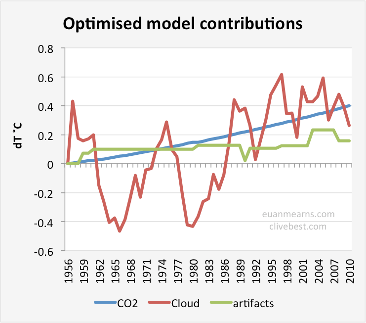
Figure 11 The relative contributions to the optimised model from dCO2, dCloud and data artifacts. It can be seen that along the time series CO2 makes the greatest contribution followed by cloud followed by artifacts.

Figure 12 The opening and closing of weather stations imparts some structure to the Tmax and sunshine data that needs to be taken into account in this and all other interpretations of such data series.
Integrating the modulus of the curves for the optimised model shown in Figure 11 along the time series and calculating the percentage contribution to the temperature record (gross dT) provides the following result:
dCO2 – 5%
dCloud – 88.5%
dArtifact – 6.5%
However, looking at the overall final contribution of each component between 1956 and 2012 (net dT; Figure 11) produces this result:
dCO2 – 49%
dCloud – 32%
dArtifact – 19%
In other words, variance in cloud cover accounts for nearly all the structure variance in UK temperature but somewhat less than half of the total temperature rise since 1956.
Discussion
The data and conclusions presented here apply only to the UK, a small island group off the West coast of Europe that currently occupies the northern end of the temperate climatic belt in a western maritime climatic setting. The polar jet stream is typically overhead and has a profound impact upon the weather regime in the UK. The NCF value of 0.54 derived from our optimised model will apply only to the UK. Other geographic locations should yield different values since they will occupy different latitudes and have different mean cloud geometries – that will fluctuate with time.
However, other localities on the Earth’s surface may be expected to display cyclical change in cloud cover that impacts surface temperature evolution. Perhaps some localities show a negative correlation between sunshine and temperature, in which case the net globally averaged effect may converge upon zero. But our analysis of global cloud cover and temperature evolution that is currently out to review suggests this is not the case [6]. Global cloud cover has fluctuated over the past 40 years and has imparted structure to the temperature record in a manner similar to that described here for the UK.
Global circulation models (GCM) that do not take into account cyclical change in cloud cover have little chance of producing accurate results. Since the controls on dCloud are currently not understood there is a low chance that GCMs can accurately forecast future changes in cloud cover and as a consequence of this they cannot forecast future climate change on Earth.
Professor Dave Rutledge from Caltech reviewed an early version of the manuscript sent to Nature and pointed out that the optimised TCR from our model = 1.28˚C was identical to the value reported by Otto et al (2013) [7]. The Otto et al work was based on a review of GCMs used in ICCP reports and applies globally. In the UK, we need to call upon increasing CO2 to produce a transient response resulting in higher temperatures to explain the observed temperature record.
Conclusions and consequences
- UK sunshine records suggest that cloud cover fluctuates in a cyclical manner. This imparts structure to the UK temperature record (confidence = very high)
- A combined CO2 radiative forcing and sunshine – surface temperature forcing model is optimised with NCF = 0.54 and TCR = 1.28˚C (confidence = medium; uncertainty unquantified)
- Our empirically constrained value for TCR = 1.28˚C is identical to the value of 1.3˚C reported by Otto et al [7]
- Our model aggregates dT over a 56 year period and provides a good fit of calculated versus observed temperature based on dCloud and dCO2 alone.
- The consequences of the above are quite profound, especially when combined with the findings of Otto et al. It removes the urgency but does not remove the long-term need to deal with CO2 emissions.
- Global cloud cover as recorded by the International Satellite Cloud Climatology (ISCCP) [8] program also shows cyclical change that helps explain the global temperature record.
- The cause of temporal changes in cloud cover remains unknown.
References
[1] MetOffice: Historic station data.(2013).at <http://www.metoffice.gov.uk/climate/uk/stationdata/>
[2] Myhre, G., Highwood, E. J., Shine, K. P. & Stordal, F. New estimates of radiative forcing due to well mixed greenhouse gases. Geophysical Research Letters 25, 2715–2718 (1998).
[3] IPCC AR5 Summary for Policy Makers (2013)
[4] Keeling, C. D. et al. Atmospheric carbon dioxide variations at Mauna Loa Observatory, Hawaii. Tellus 28, 538–551 (1976).
[5] Kusterer, J. M. NASA Langley Atmospheric Science Data Center (Distributed Active Archive Center). (2008).at <https://eosweb.larc.nasa.gov/index.html>
[6] Effect of Cloud Radiative Forcing on Climate between 1983 and 2008, C. H. Best and E. W. Mearns (under review)
[7] Otto, A. et al. Energy budget constraints on climate response. Nature Geoscience 6, 415–416 (2013)
[8] The International Satellite Cloud Climatology Project (ISCCP) <http://isccp.giss.nasa.gov/>
[9] Richard P. Allan, Combining satellite data and models to estimate cloud radiative effects at the surface and in the atmosphere, RMetS Meteorol. Appl. 18: 324–333, 2011
Note: This article was originally posted at:
Biosketches:
Euan Mearns has a PhD in Geology / Isotope Geochemistry and Clive Best has a PhD in High Energy Physics. Further bio information can be obtained at:

It is useful to know that cloud variability may have such a significant effect. But it is highly unlikely that clouds and CO2 alone explain climate change. The literature is full of similar studies that suggest significant influence from other factors. Thus the conclusions drawn here are overreaching.
Yes, it is “unlikely that clouds and CO2 alone explain climate change” but congratulations are in order to Euan Mearns and Clive Best for having the courage to publish information that the gatekeepers of knowledge seek to hide from the public!
With kind regards,
Oliver K. Manuel
Former NASA Principal
Investigator for Apollo
The article would have more credibility if the authors had stated WHY Nature had rejected their submission.
They did.
Agreed. It was not our intention to give that impression. But it was our intention in saying “CO2 alone” that there was not a lot of room for large net positive feedbacks. Other factors to which you refer may actually make their mark by influencing cloud cover. For example a change in ocean circulation or a change in the spectral output from the Sun
I performed an analysis similar to yours using Mauna Loa CO2 concentration data and HadCrut4 yearly global average surface temperature data over the period 1850-2012. I concluded, assuming all long term warming effects were due to CO2, that an Upper Bound for TCR was 1.6 deg C, consistent with your results. I also found that a 62 year temperature cycle in the HadCrut4 data with amplitude of +/- 0.15 deg C captured major features of the multi-decadal oscillations in the data. Year to year variations were not addressed and were considered to be noise in the data. Others have suggested such multi-decadal oscillatory behavior in yearly global average surface temperature is due to PDO and AMO, which also affect cloud cover.
Cleaner air as the result of clean air legislation.
http://sunshinehours.wordpress.com/2012/12/05/uk-tmax-versus-sunshine-are-well-correlated-cleaner-air-more-sunshine/
“Staggering 20% Increase in Surface Solar Radiation Due to Cleaner Air In Just One Decade”
http://sunshinehours.wordpress.com/2013/08/19/staggering-20-increase-in-surface-solar-radiation-due-to-cleaner-air/
“reducing aerosol pollution is driving the Insolation Brightening phenomenon”
http://sunshinehours.wordpress.com/2013/03/14/cleaner-air-more-sunshine/
etc
http://sunshinehours.wordpress.com/2013/01/17/sunshine-way-up-in-usa-from-1996-to-2011/
http://sunshinehours.wordpress.com/2012/05/15/more-sunshine-in-the-netherlands/
@ Harold Doiron – interesting. I think you’ll find over the time interval a small incremental change in cloud cover accounts for some of the warming that would drive down your TCR. The real issue here is how IPCC in AR5 get away with leaving the upper bound at 4.5˚C. Otto et al point to 1.3˚C and manage to drive the lower bound down to 1.5˚C. But why not 1.3˚C? And what evidence exists to warrant any figure >>1.5˚C?
” The real issue here is how IPCC in AR5 get away with leaving the upper bound at 4.5˚C”
Answer is they don’t. You are confusing ECS and TCS
http://tallbloke.wordpress.com/2012/02/13/doug-proctor-climate-change-is-caused-by-clouds-and-sunshine/
Check out above. The data isn’t that difficult to find, analyse.
http://tallbloke.wordpress.com/2012/02/13/doug-proctor-climate-change-is-caused-by-clouds-and-sunshine/
The data isn’t that difficult to analyse and interpret. Even a citizen can do it. Not that he will make any money from the effort, which is the second point of academia.
From the paper I read “so applying the value of the Planck response (3.5 Watts/m2/˚C) we get a CO2 climate sensitivity of 1.05˚C.”
Sorry, this is nonsense. The climate sensitivity of CO2 is unknown, since it is impossible to measure it. We cannot do controlled experiments on the earth’s atmosphere. The assumption that convection plays no part in compensating for any radiative imbalance makes this estimation meaningless.
Since no-one has detected a CO2 signal in any modern temperature/time graph, this fact gives a strong indication that the climate sensitivity of more CO2 added to the atmosphere from current levels is indistinguishable from zero.
It takes time Jim. One still have to pay the CO2 lip service, but less and less.
Edim, you write “It takes time Jim. One still have to pay the CO2 lip service, but less and less.”
Again, sorry, Edim, I don’t think we have any time left. Science, physics, is being raped by the warmists. I am afraid we have past the point in time when drastic action needs to be taken.
“Pierre, only the net flux counts for the heat (energy) transfer.”
Sure, so what? It’s not the magnitude of the net radiative energy transfer from surface to atmosphere that’s at issue. It’s rather the greenhouse effect and Jim Cripwell’s claim that CO2 “doesn’t add joules to the atmosphere” that is at issue. CO2 does add joules to the surface. Whatever the net flux is, it results from the difference from the gross fluxes up and down (minus sensible and latent fluxes). The gross upwelling flux is a function of surface temperature only. It must closely balance the gross dowelling flux. This latter flux is huge because of clouds and greenhouse gases. Hence the surface must be much warmer (about 33 degree °C) to compensate not only for the solar flux but also the for huge gross downwelling flux.
The Planck response is simply the average increase in black body radiation following a 1C increase in surface temperature whatever the cause and does not depend on CO2. For example it could also be a response to an increase in temperature caused by solar radiation or less clouds.
S = sigma.T^4 –> DS/DT = 4.sigmaT^3. 4 sigma Teff^3 works out at about 3.5 W/m2/C.
Earth’s surface is in direct contact with the atmosphere and it’s cooled mostly non-radiatively. The atmosphere, on the other hand, is cooled exclusively by radiation to space (the so-called GHGs and clouds).
Clive, you write “For example it could also be a response to an increase in temperature caused by solar radiation or less clouds.”
This is simply not true. When CO2 supposedly increases global temperatures, there are no new joules added or subtracted from the heat reaching the earth’s surface. For the examples you chose, the number of joules changes.
A bit of a nit but clouds have a third forcing impact in direct absorption of SW that can effect Planck response.
http://edberry.com/SiteDocs/PDF/Climate/KimotoPaperReprint.pdf
Jim Cripwell wrote: “When CO2 supposedly increases global temperatures, there are no new joules added or subtracted from the heat reaching the earth’s surface.”
The downwelling longwave radiation hitting the surface averages 333W/m^2. This is more than twice the post-albedo incident solar energy. Greenhouse gases and clouds are responsible for this. The surface must warm to balance this and emit as much power as it receives. Latent and sensible heat isn’t nearly enough. In any case, the 396W/m^2 surface radiation is verified empirically.
Pierre, you write “The downwelling longwave radiation hitting the surface averages 333W/m^2.”
Please correct me if I am wrong. So far s I am aware, the change in joules from a change in the solar constant, or cloud cover has been measured. The change in downwelling longwave radiation as the amount of CO2 increases has not been measured. That is a major difference.
Pierre-Normand,
Then the radiative heat exchange surface->atmosphere is:
396 – 40 – 333 = 23 W/m2
Convection is 17 and evaporation 80 W/m2, according to this budget:
http://www.cgd.ucar.edu/cas/Topics/Fig1_GheatMap.png
Jim Cripwell, you had written: “When CO2 supposedly increases global temperatures, there are no new joules added or subtracted from the heat reaching the earth’s surface.”
This is a categorical claim. I though you had some positive ground for advancing it. Is you argument simply that only clouds and water vapor can account for the totality of the 333W/m^2 and that you don’t personally believe CO2 (and methane, etc.) can contribute any fraction of it, for no particular reason? Is there some “null hypothesis” according to which H2O is a greenhouse gas and CO2 isn’t?
That’s correct Edim. But my point just is that the greenhouse effect accounts for the Earth surface being much warmer (about 33°C) than it would need to be in order just to upwell the same longwave power as it receives (mostly shortwave) from the Sun if the atmosphere were transparent. Jim’s claim that CO2 “adds no joules” to the surface is at best meaningless, at worst false. It’s responsible in part for the huge downwelling power. His claim that the mechanism involves “raping physics” is just bizarre.
Pierre, what huge downwelling power? It’s only ~23 W/m2 and it’s upwelling, as you agreed.
Pierre, I said please correct me if I am wrong. I am wrong, thank you.
Edim, you only are considering the net radiative flux from surface to atmosphere. This flux, of course, merely balances out the small non-radiative fluxes (sensible + latent), modulo the part that escapes through the atmospheric window (40W/m^2). The gross downwelling flux is huge. It is more than twice the shortwave solar flux. So, the surface must warm 33°C (compared with the no greenhouse effect case) in order for the upwelling flux to balance out the equally huge downwelling flux. Were it not for the greenhouse gases (and clouds), the downwelling flux would be zero and the upwelling flux would only be equal to the post-albedo solar flux minus some very small sensible flux (with no latent flux since, ex hypothesi, there would no water vapor).
Jim Cripwell, I am still undecided whether you are wrong or net even wrong. You just aren’t making sense.
Pierre, only the net flux counts for the heat (energy) transfer.
Clive.
Cripwell will never get this as its fundamental physics
@Pierre-Normand | November 15, 2013 at 10:40 am |
“The gross downwelling flux is huge.”
Not under all conditions. DWLR at Zenith on a 35F clear day at ~local noon, -40F. Which is around 160 some watts/sq meter.
You can measure it with a hand held IR thermometer (get the -70F minimum rage model).
Edim remarked: “Pierre, only the net flux counts for the heat (energy) transfer.”
My response was appended above.
http://ca.news.yahoo.com/japan-drastically-scales-back-co2-emissions-cut-target-002021962–business.html
Jim Cripwell | November 15, 2013 at 7:03 am | Reply
F”rom the paper I read “so applying the value of the Planck response (3.5 Watts/m2/˚C) we get a CO2 climate sensitivity of 1.05˚C.””
It’s not nonsense but it’s certainly not an experimental result. Factors other than CO2 that potentially change surface temperature must be assumed and then subtracted to leave CO2 isolated. The devil is in the assumptions.
Agreed. When I set out to find someone to help me with this I was asking for a “back of the envelope” type calculation. Confronted with a curve of varying sunshine I really had no clue whether or not this would convert to sensible dT. At one point it looked like we could explain whole dT by DSun/Cloud, but we couldn’t. So we thought, ah ha, lets stick CO2 in there as well. Its quite clear that if you add other “influences” such as methane, land use changes etc. then this reduces the role of CO2 in our model. Geologists are driven by “gut feel” and my gut feel on this one is that the net effect (CS / TCR / ECS) for CO2 all lie close to 1˚C.
well the problem is you are treating sunshine as a forcing, when it could be coupled with the feedback. Also this is not global, and a particular region is not constrained by global energy balance.
@euanmearns
Agreed. But since you have no attribution for cloud change it could be the change in CO2 that is driving the change in cloud cover. My feeling is that increased DWLIR from more CO2 doesn’t directly raise surface temperature significantly anywhere there is abundant water on the surface to evaporate. DWLIR only penetrates a few microns into liquid before it is completely absorbed. This drives evaporation higher and produces a well known “cool skin layer” on the ocean surface where the top 1mm is 0.5C cooler than the water below it. This has another known effect called lapse-rate feedback which is basically restated as clouds forming at higher altitude but at the same dewpoint temperature. A cloud top at the same temperature but higher altitude has a less restricted radiative path upward to space and a more restricted radiative path back to the surface. The net result is that there’s little surface heating due to non-condensing greenhouse gases over the ocean but rather clouds will form about 100 meters higher in the atmosphere for every CO2 doubling. Given that clouds have a net negative feedback (deserts have higher mean annual temperatures than non-desert at the same latitude & altitude) it means that non-condensing greenhouse warming is only significant over dry land. The kicker is that frozen land is dry land so we find the greatest non-condensing GHG signature at higher latitudes in the northern hemisphere where there’s much more land surface that is frozen for at least part of the year. Increasing ocean heat content is explained by warmer runoff from the continents and that method of adding heat to the ocean would not be detectable passing through the first 700 meters of the ocean by ARGO as mixing & sinking occurs in shallow water on continental shelf where the buoys are absent. The buoys would just mysteriously see OHC rising below 700 meters. In fact that is what we observe and there’s no small amount of consternation about the mechanism for deep ocean heating that is undetectable passing through the mixed layer. :-)
I must disagree with your statement, “The climate sensitivity of CO2 is unknown, since it is impossible to measure it.” If you mean Equilibrium Climate Sensitivity (ECS), a ficticious, unverifiable, misguided and ill-advised numerical simulation way to understand the true effects of CO2, I agree. But Transient Climate Response (TCR) is a much more reasonable and realistic climate simulation method to compute global surface temperature changes as atmospheric CO2 concentration slowly rises and eventually will fall, as we run out of economically recoverable fossil fuels in the next 100-200 years.
Since I don’t believe time and money should be wasted on un-validated climate model simulations, I prefer to use the term Transient Climate Sensitivity (TCS) for extractions of the CO2 climate sensitivity from actual data, similar to the approach of Mearns and Best, rather than TCR climate model simulations based on a ficticious 1% per year rise in atmospheric CO2 concentration, that is about twice the actual current rise rate. However, as an experienced dynamics modeler of complex systems, I believe the official TCR simulation CO2 rise rate is slow enough to essentially make the TCR value equivalent to Transient Climate Sensitivity (TCS) extracted from actual data. If the net CO2 climate sensitivity embedded in a climate simulation model is ever to be validated, the simulation solution must first be shown to agree with the available long term global average surface temperature trends using actual atmospheric CO2 concentration data as a forcing function.
Therefore, why not just use the actual data from 1850 AD to the present time to determine the climate sensitivity of CO2? The fact that climate science has studied CO2 climate sensitivity for over 30 years and spent billions of research dollars, without narrowing the uncertainty range of CO2 climate sensitivity (ECS) from 1.5 to 4.5 deg C, indicates to me that removing uncertainty in the ECS prediction was never the goal of the research. The available data supports the lower end of the uncertainty range (kept in the official uncertainty band, I assume, for ethical cover), and the higher values result from un-validated climate simulation models that should be ignored in forecasting and related public policy decision-making with potentially severe adverse consequences.
Mearns and Best demonstrate in Figure 8, how using a value of TCR = 3 deg C, results in the predicted long term temperature rise departing from actual data trends. However, when one applies a similar CO2 climate sensitivity extraction approach to the Hadcrut4 global average surface temperature data over the 163 years from 1850 AD thru 2012, a TCR value as high as 2 deg C causes a marked rise in T_calc above the HadCrut4 data. Using a similar CO2 climate sensitivity extraction approach as Mearns and Best, and assuming all long-term warming effects were due to CO2 rise in the atmosphere, I determined an Upper Bound for TCR = TCS = 1.6 deg C based on the yearly average HadCrut4 and Mauna Loa atmospheric CO2 concentration data since 1850 AD. This is a very easy and straight-forward analysis to perform. The longer trend T_calc function I used to fit HadCrut4 data over the 163 yr period and determine my Upper Bound for TCS was:
T_calc = Initial HadCrut4 Temp Anomaly+TCS*LOG[CO2(yr)/280]/LOG(2)
Harold, you write ” I prefer to use the term Transient Climate Sensitivity (TCS) for extractions of the CO2 climate sensitivity from actual data.”
In principle, I agree. However, we cannot do controlled experiments on the earth’s atmosphere, and we do not know all the natural variations. So I fail to see how you can extract a value for climate sensitivity at the present time. How can you prove whether any observed temperature change was caused by a change in CO2 concentration?
Harold, in a sea of disparate opinion, we seem to be on the same page. I gave a talk on this at The University of Aberdeen earlier this week and made the point you make above that it was IMO outrageous that after so much research and money the result was a range in uncertainty totally unfit for any policy framework. Some in the audience seemed unable to grasp this simple point and seemed offended that anyone should dare to point out that this King has no clothes.
Jim Cripwell,
I believe at this point we should use available data rather than un-validated climate models to narrow the uncertainty range regarding climate sensitivity to CO2. My “conservative” Upper Bound estimate for TCS < 1.6 deg C was achieved assuming all long-term warming in the 163 years of available data was due to CO2. Any other long-term warming effects (such as continued natural warming from The Little ice Age) would tend to reduce the upper bound determination, as well as, best estimate for TCS which I believe is on the order of 1.1 deg C. The only situation that would invalidate very my very simplistic Upper Bound extraction for TCS is some long-term effect, such as solar variation, that had a cooling effect over most of the 163 period, and that would tend to cause an under-estimation of the CO2 TCS value. This remote possibility can be assessed with available solar output data. IPCC AR5 makes an attempt to do this but they use 1750 AD as a starting point for their analysis, 100 years before the HadCrut4 data record begins, so I worry about the quality of the data they used.
As other authors have found (Ring et. al. (2012) for example), Quasi-Periodic Oscillations (QPO) in the global average surface temperature record tend to average to near zero over a long period of time as do variations in aerosols, effects of volcanoes, etc. I agree with Mearns' comment to my one of my posts herein, that my 1.6 deg C Upper Bound estimate for TCS can be lowered with more data analysis. However, I was trying to do something quick and simple to establish a conservative Upper Bound and evaluate whether that conservative upper bound gave us anything to worry about, eg. "Can we get rid of all the alarmism about AGW?" Many papers published in the last couple of years are concluding that CO2 ECS climate sensitivity is near the lower range of the official IPCC ECS uncertainty range of 1.5 to 4.5 deg C. Using the results of IPCC AR4 Table 8.2 where results of TCR and ECS simulations with over 20 different climate models were provided, an average value for
TCR/ECS = 0.56
Therefore, the IPCC 1.5 – 4.5 deg C uncertainty range for ECS can be mapped into an estimated uncertainty range for TCR of 0.84 to 2.5 deg C. Using actual data, the 2.5 deg C IPCC derived upper limit for TCR can be shown to be obviously too high. Mearns and Best, and many other recent and totally independent studies are consistent with my simple conservative upper bound extraction for TCR = TCS < 1.6 deg. What PROBLEM is created by TCR = TCS as high as 1.6 deg C? What, Where, When and by How Much will any specific PROBLEM (harmful deviation from normal) arise? Let's put this AGW issue to bed!!
Harold H. Doiron
Your approach to establishing an upper limit for the 2xCO2 TCR based on actual physical observations makes sense to me.
You arrive at an upper limit of 1.6ºC based on global data.
As you wrote Jim Cripwell:
Based on the UK record alone, the Mearns + Best study arrives at an empirically constrained value for TCR = 1.28˚C, adding:
These results check out fairly well with those of several independent (at least partially) observation-based studies, which suggest a mean value for 2xCO2 climate sensitivity at equilibrium (ECS) of around 1.8ºC.
Lewis (2013): 1.0C to 3.0C
Berntsen (2012): 1.2C to 2.9C
Lindzen (2011): 0.6C to 1.0C
Schmittner (2011): 1.4C to 2.8C
van Hateren (2012): 1.5C to 2.5C
Schlesinger (2012): 1.45C to 2.01C
Masters (2013): 1.5C to 2.9C
The average range of these recent studies is 1.2°C to 2.4°C, with a mean value of 1.8°C, well below the model-derived estimates used by IPCC of 1.5ºC to 4.5ºC, with a mean value of 3ºC.
As Cripwell has noted elsewhere, ECS itself is a rather nebulous virtual concept, which cannot be determined empirically, in any case.
As you wrote Cripwell:
Comment reposted with corrected formatting
Harold Doiron
Your approach to establishing an upper limit for the 2xCO2 TCR based on actual physical observations makes sense to me.
You arrive at an upper limit of 1.6ºC based on global data.
As you wrote Jim Cripwell:
Based on the UK record alone, the Mearns + Best study arrives at an empirically constrained value for TCR = 1.28˚C, adding:
These results check out fairly well with those of several independent (at least partially) observation-based studies, which suggest a mean value for 2xCO2 climate sensitivity at equilibrium (ECS) of around 1.8ºC.
Lewis (2013): 1.0C to 3.0C
Berntsen (2012): 1.2C to 2.9C
Lindzen (2011): 0.6C to 1.0C
Schmittner (2011): 1.4C to 2.8C
van Hateren (2012): 1.5C to 2.5C
Schlesinger (2012): 1.45C to 2.01C
Masters (2013): 1.5C to 2.9C
The average range of these recent studies is 1.2°C to 2.4°C, with a mean value of 1.8°C, well below the model-derived estimates used by IPCC of 1.5ºC to 4.5ºC, with a mean value of 3ºC.
As Cripwell has noted elsewhere, ECS itself is a rather nebulous virtual concept, which cannot be determined empirically, in any case.
As you wrote Cripwell:
This would put the upper limit for ECS, based on your study, at 1.6/0.56 = 2.9ºC, on the unlikely basis that all warming since 1850 can be attributed to CO2.
The several independent studies cited above also arrive at upper limits for ECS in this magnitude or slightly lower, rather than the 4.5ºC, now being claimed by IPCC.
But, unfortunately, it is the upper ECS range, which is used by IPCC to paint the “CAGW” horror scenarios, as outlined in its AR4 and AR5 reports.
So the whole CAGW hysteria is based on theoretical model-derived estimates, which are arguably grossly exaggerated, at best. And, as Cripwell writes, the theoretical no-feedback 2xCO2 ECS as estimated by Myhre et al. can also not be corroborated by observational data, so the whole horror scenario rests on long-range projections supported by model-derived parameters backed by theoretical deliberations, rather than empirical evidence.
To me the key question that needs to be answered is simply: “does CO2 have a significantly high effect on our climate to represent a severe potential threat to humanity and our environment or not?”
The IPCC ECS range of 1. 5ºC to 4.5ºC does not answer this question.
A recent Tol study concludes that GH warming experienced to date has had a net beneficial impact for humanity, and that future warming up to around 2.2º to 2.5ºC would also have positive impacts on balance. So a problem could arise for humanity if future GH warming were to significantly exceed 2.5ºC.
If the ECS is constrained to 2.5ºC or less, as your estimate seems to indicate, we have no problem of overheating our planet with the remaining fossil fuel resources.
And that is essentially the key “take home” from all these recent studies.
Max
Re: Mearns “Interpretation of UK temperatures since 1956”
The most powerful feedback in Earth’s climate is albedo because it gates the Sun on and off. Earth’s climate vacillates between two major climate states, predominantly the cold state (Snowball Earth) when the surface albedo dominates to turn the Sun off, and the rarer warm state like the present when the surface is dark, the ocean liquid, and cloud albedo dominates. In the warm state, cloud cover is a positive feedback to TSI and a negative feedback to surface (GAST). Hence, cloud cover amplifies sunlight and at the same time mitigates warming from any cause. As the surface warms, humidity increases. That humidity on average guarantees additional cloud cover because on average the atmosphere has a surplus of CCNs. That effect is known by the observation that clouds form reliably with increasing surface temperature and dissipate with increasing sunlight, as in the diurnal effects over the ocean. This is the mechanism, and not the Greenhouse Effect, which regulates Earth’s climate. Cloud cover follows surface temperature to mitigate it. The Greenhouse Effect is dominantly caused by water vapor, and in the cold state the atmosphere is so dry that the Greenhouse effect is turned off. Similarly, atmospheric CO2 follows surface temperature because of Henry’s Law of Solubility. CO2 is readily dissolved in water, and its solubility decreases as temperature increases. As a result, Earth’s atmospheric CO2 concentration does not lead but follows GAST. The causation arrow is the reverse of that in AGW. GAST causes atmospheric CO2, not the reverse. Earth’s temperature follows the intensity of solar radiation, i.e., it follows the Sun, the heat being integrated in and distributed by the dark, absorbent ocean, especially in the tropics. The primary integration time constants are about a millennium due to the heat and carbon pump known as the thermohaline circulation, with secondary time constants of about 150 and about 50 years. The Sun is the source, and neither the Greenhouse Effect, formerly better known as the Callendar Effect, nor clouds.
Mearns and Best are just beginning the discovery of climate in a closed community. It is different than the AGW dogma, so they can’t be published.
Science and Nature reject many papers and have for years. They want things that are flashy and of high general interest. They also want to represent many different fields including the occasional social science paper which also limits how many they can accept. Papers can be excellent work but not significant or flashy enough and not get accepted. Or they can be of low general interest or too long or technical and not get accepted.
In other journals, a good paper getting rejected and taking years to get through peer review can be an indicator of bias and I do think this happens, especially in climate science. In Science or Nature, I’m sure this happens too but it is just very difficult to get things into these journals. However, I do think some people tend to get over-represented in Science or Nature and this probably depends on the reviewers and editors they have in place during that time period and can definitely have an effect. My main point is that a good paper not making it into Nature is not evidence by itself of bias and I did not see Judith or Clive making that argument.
Bill, 11/15/13, 8:00 am:
The ultimate test for scientific models in Modern Science, though not Post Modern Science, is its predictive power. The ultimate test in PMS, but not MS, is its publication in approved, peer-reviewed, professional journals. “Publish or perish”. Climate science is firmly camped in PMS, and it’s not alone.
Read the lament of Richard Horton, Editor of the Lancet, on peer-review. He spoke in a rare moment of rational honesty, and it is available in several places on Judith Curry’s blog.
Yes, they publish everything that is alarmist and everything that meets the consensus, and everything that comes from recognized consensus people, and it does not matter much to them if the papers are good or bad. Studies have been done where they submitted papers and waited and submitted the same papers with a recognized name and the second got published. They do not publish papers that disagree even when they are really excellent.
Climate Model output for the past ten thousand years is a ten thousand year old Hockey Stick. Climate Model output goes up and down with CO2 and there are no downs in the past ten thousand years for CO2.
Earth temperature goes up when Land Ice is receding and Earth temperature goes down when Land Ice is advancing. Land Ice Advances during and after the warm times because that is when the snow falls. Land Ice Retreats during and after a cold time because that is when there is not enough snowfall to replace what melts every summer.
They add the ice on land after it gets cold and that is when the wet water is not available because it is covered with Sea Ice. They remove the ice on land after it gets warm and the snowfall has already started again.
They do not have the Polar Ice Cycles right yet.
I do put most of my trust in the Ice Extent.
Clouds also help. When Oceans are warm and the snow is falling it is from increased Cloud Cover. When oceans are cold and frozen and snow is not falling, it is with less Cloud Cover.
It is IR that does most of the cooling of the Earth and most of that from the Water Vapor. CO2 helps a little bit. CO2 is only a trace gas and Water Vapor is abundant. This has NO SET POINT. Look at data for the past 600 million years. That is how temperature varies without the Polar Ice Cycles.
It is the Polar Ice Cycles that have a Set Point and provide the thermostat and forcing for narrow temperature bounds.
Look at the Ice Core Data for the past 800 thousand years. That is how temperature varies as the Polar Ice Cycles are evolving.
Look at the Ice Core Data for the past ten thousand years. That is how temperature varies with the Modern Polar Ice Cycles.
Temperature varies differently as the Polar Ice Cycles changes and moved into the modern pattern.
A molecule of man-made CO2 per ten thousand molecules of other molecules (including natural CO2) will not kick us out of this well bounded temperature range.
If CO2 does cause any warming, it will melt more Polar Sea Ice and increase the Snowfall. The temperature bounds will not be broken.
” They want things that are flashy and of high general interest.”
Heh.
So a front cover is warranted for a paper that uses dubious maths to smear warming in a small part Antarctica across the entire continent (“it’s worse than we thought!”, or perhaps “changes our understanding of the temperature response of one – unpopulated – continent”), yet a paper that shows other factors than CO2 may be important (“it’s not as bad as we thought” or perhaps “changes our understanding of the temperature response of one – populated – continent, with indications it also affects global response”) doesn’t even warrant being published?
Doesn’t seem reasonable to me. Perhaps the authors needed to include a graphic of the UK, covered in red ink and with a caption like “UK temperature increases over 40 years” to get published – that’d “flash it up” enough, eh?
Sorry, but it really seems to me that Nature is no better than the MSM – they want dramatic, scarey headlines. If so, that is their choice – but I wonder what this will eventually do (if not has already done) to it’s reputation as “prestigious”, “trustworthy”, “high impact” etc. If they are indeed “taking sides” in a scientific debate, they certainly deserve any and all hits to their reputation.
Kneel
An even better but less scary headline would be to point out the facts:
‘Uk temperature back to where it was 40 years ago’
http://noconsensus.wordpress.com/2010/01/06/bah-humbug/
Tonyb
Tony, that’s scary.
1963 in the UK was f’in cold.
Hello Jeff.
Do you not consider atmospheric mass as relevant to the so called greenhouse effect ?
Stephen Wilde, 11/15/2013, 8:40 am, asks Do you not consider atmospheric mass as relevant to the so called greenhouse effect ?
While AGW gives me great discomfort, the Greenhouse Effect does not. The difference between Earth’s warm and cold states is due in part to the absence of any GE in the latter. When the GE is operative, i.e., out of the deep cold state, it is dependent on the relative mass of the greenhouse gases, and especially water vapor. If the atmospheric mass could increase significantly, then the mass of GHGs would increase, and that would cause an increase in the GE. Absorption of CO2 in the atmosphere is approximately logarithmic over the full range of Radiative Transfer calculations, but that is due to the fact that 100% CO2 isn’t dense enough to show the saturation in Beer’s Law. If the mass of the atmosphere were much greater, and hence the partial pressure of CO2 correspondingly greater, the logarithmic effect would fade into saturation with increasing relative CO2 concentration.
+1 again for Glassman
It’s a shame that common sense is so rare it deserves a +1 to help it stand out.
+1 for a glass of beer, man.
The Land Ice Extent is much more in a Little Ice Age and in all the cold periods. The Land Ice Extent is much less in a Roman or Medieval or Modern warm time and in all the warm times.
They did the story above without using the word Albedo even once.
Earth Temperature is ALWAYS in phase with Land Ice Extent.
They do not understand Polar Sea Ice Cycles and how it always snows more when the Polar Waters are warm and wet and it always snows less when the Polar Waters are cold and frozen.
Temperature changes with Albedo. They don’t get this yet.
Land / water / ice surface area changes are not relevant to the UK since 1956. We are simply working out a “spontaneous” energy balance over UK and find that dCloud and dCO2 can explain much of it in this 56 year period. It just so happens that the transient climate response for our optimised model was the same as that estimated by Otto et – and that number was global.
Earth Temperature has a set point and powerful forcing to keep temperature bounded close to the set point.
The temperature that Polar Sea Ice Melts and Freezes is the only set point. It snows when it is exceeded and water is wet. It don’t snow when it is not exceeded and water is covered by sea ice.
All the other forcing’s can push temperature around, in bounds, but none of them can push temperature out of bounds. When we are warm, it always snows and then Earth gets cold. When we are cold, it always snows less and then Earth gets warm.
This is supported by the Greenland and Antarctic Ice Core Data. Look at my web site.
Start here, 2700-2600 BC was very warm in the temperate zone (extratropics), and 1300-1200 BC was very cold in the temperate zone. Greenland was doing the complete opposite:
http://smpro.ca/crunch/GISP2Civil.png
hmm the hockey stick was not a reconstruction of greenland temperature. why has it been spliced onto the end of a graph of greenland temperature?
@lolwot
The point is that Greenland temp’s have been used as a proxy for temperate zone temp’s, but they move in opposition.
Most of this moves in opposition to CET:
http://www.21stcentech.com/wp-content/uploads/2012/07/Greenland-ice-core-data.png
http://climexp.knmi.nl/data/tcet.dat
Jeff, you wrote:
The ultimate test for scientific models in Modern Science, though not Post Modern Science, is its predictive power.
I predict that the next ten thousand years will follow the pattern of warming and cooling that we have had for the past ten thousand years with a Polar Sea Ice Set Point and the same Tight Bounds.
+1 for Glassman
It is clear to me that there must be temperature self regulation on Earth due to 70% coverage in oceans. Otherwise the oceans would have boiled away billions of years ago as the sun brightened by 70%. AGW relies on positive H2O feedbacks (F) as high as 2 W/m2/C. The sun has brightened by 30% over 4 billion years
Black body radiation from the Earth’s surface is the primary negative feedback to any temperature rise DT.
DT =DS/(4σT3 -F)
The basic problem is that if the temperature falls sufficiently so that 4σT3= F then a singularity occurs ~1.5 billion years ago for F=2 w/m2/C. Therefore F must be zero or positive.
Clouds and Ice albedo must play a major role in maintaining temperatures for the oceans within the liquid water phase. Clouds play the same role on Earth as the white daisies do on Lovelock’s Daisy World !
Clive Best, 11/15/13, 5:11 pm, says, Black body radiation from the Earth’s surface is the primary negative feedback to any temperature rise ΔT.
While that is not a feedback in any sense in which I used the word with respect to cloud cover, the statement is not without support in climate science literature, where the concept is thoroughly confused. Clauses like “treated as a feedback” or “considered a feedback” bury uncertainty in climate modeling even deeper behind the passive voice.
IPCC alone has three different definitions of feedback. IPCC’s Glossary definition, while reminiscent of the original, is steeped in ambiguity. AR4 Glossary, “Climate feedback”, p. 946. Another IPCC definition turns feedback as a signal into feedback as mere correlation. TAR, Figure 7.6, p. 445. The third distinguishes feedbacks from forcings and responses, divorcing the concept of feedback from the climate model and converting it into a programmer’s climate modeling choice. TAR, Appendix 6.1, Elements of Radiative Forcing Concept.
On that foundation, IPCC confesses,
>>”Since the TAR a number of studies have investigated the relationship between RF and climate response, assessing the limitations of the RF concept; related to this there has been considerable debate whether some climate change drivers are better considered as a ‘forcing’ or a ‘response’. Bold added, citation deleted, AR4, ¶2.2, Concept of Radiative Forcing, pp. 133-4.
Little can be accomplished in this Post Modern Science realm, where, as Popper its creator famously said, “Definitions do not matter.” When investigators wanted to estimate climate sensitivity from recent satellite data, they had to settle on a definition for feedback. Lindzen & Choi (2011) stood out from the group by choosing the original, systems science meaning. (The only problem with their results was that they arbitrarily restricted feedback to linear regression instead of higher order regression.)
My remarks are based, as they must be, solely on systems science, where the notion of feedback first appeared on solid theoretical grounds (i.e., Modern Science). That is where Hansen et al., (1984) discovered the pioneering electronics of H. W. Bode to introduce feedback into climate modeling:
We use procedures and terminology of feedback studies in electronics (Bode. [Network Analysis and Feedback Amplifier Design] 1945) to help analyze the contributions of different feedback processes. Id., p. 131.
Unfortunately the textbook definitions of feedback in system science all seem to turn on a system block diagram, as did the Lindzen & Choi model. That is comfortable for engineers, but an unnecessary restriction because science leaves the selection and arrangement of elements for the model of a physical system to the investigator. Here is my own, block-diagram free, systems science based definition of feedback:
Feedback is a signal generated within a system that modifies the system inputs. A system is any complete interconnection of entities with observable input and output signals. A signal is any parameter or quantity that can be measured and transmitted within a system, including acceleration, capacitance, color, conductance, dielectric strength, displacement, elasticity, energy, extent, flow, force, frequency, inductance, information, intensity, material, period, permeability, polarization, potential, power, pressure, rate, resistance, temperature, time, or volume, or a combination of such parameters.
In climatology, whether the Planck response is a feedback is undecidable. In systems science, it is not a feedback, but belongs to the general class of system responses or outputs. A sufficient reason that the Planck response is not a feedback is that it does not modify the inputs to the climate system, at least in any imaginable, well-designed climate model. Cloud cover does modify the inputs to climate. It modifies the solar radiation supply to Earth’s climate, making it the most powerful of all climate feedbacks.
Clive Best, 11/15/13, 5:11 pm, says, Black body radiation from the Earth’s surface is the primary negative feedback to any temperature rise ΔT.
While that is not a feedback in any sense in which I used the word with respect to cloud cover, the statement is not without support in climate science literature, where the concept is thoroughly confused. Clauses like “treated as a feedback” or “considered a feedback” bury uncertainty in climate modeling even deeper behind the passive voice.
IPCC alone has three different definitions of feedback. IPCC’s Glossary definition, while reminiscent of the original, is steeped in ambiguity. AR4 Glossary, “Climate feedback”, p. 946. Another IPCC definition turns feedback as a signal into feedback as mere correlation. TAR, Figure 7.6, p. 445. The third distinguishes feedbacks from forcings and responses, divorcing the concept of feedback from the climate model and converting it into a programmer’s climate modeling choice. TAR, Appendix 6.1, Elements of Radiative Forcing Concept.
On that foundation, IPCC confesses,
>>”Since the TAR a number of studies have investigated the relationship between RF and climate response, assessing the limitations of the RF concept; related to this there has been considerable debate whether some climate change drivers are better considered as a ‘forcing’ or a ‘response’. Bold added, citation deleted, AR4, ¶2.2, Concept of Radiative Forcing, pp. 133-4.
Little can be accomplished in this loosey-goosey, Post Modern Science realm, where, as Popper its creator famously said, “Definitions do not matter.” When investigators wanted to estimate climate sensitivity from recent satellite data, they had to settle on a definition for feedback. Lindzen & Choi (2011) stood out from the group by choosing the original, systems science meaning. (The only problem with their results was that they arbitrarily restricted feedback to linear regression instead of higher order regression.)
My remarks are based, as they must be, solely on systems science, where the notion of feedback first appeared on solid theoretical grounds (i.e., Modern Science). That is where Hansen et al., (1984) discovered the pioneering electronics of H. W. Bode to introduce feedback into climate modeling:
We use procedures and terminology of feedback studies in electronics (Bode. [Network Analysis and Feedback Amplifier Design] 1945) to help analyze the contributions of different feedback processes. Id., p. 131.
Unfortunately the textbook definitions of feedback in system science all seem to turn on a system block diagram, as did the Lindzen & Choi model. That is comfortable for engineers, but an unnecessary restriction because science leaves the selection and arrangement of elements for the model of a physical system to the investigator. Here is my own, block-diagram free, systems science based definition of feedback:
Feedback is a signal generated within a system that modifies the system inputs. A system is any complete interconnection of entities with observable input and output signals. A signal is any parameter or quantity that can be measured and transmitted within a system, including acceleration, capacitance, color, conductance, dielectric strength, displacement, elasticity, energy, extent, flow, force, frequency, inductance, information, intensity, material, period, permeability, polarization, potential, power, pressure, rate, resistance, temperature, time, or volume, or a combination of such parameters.
In climatology, whether the Planck response is a feedback is undecidable. In systems science, it is not a feedback, but belongs to the general class of system responses or outputs. A sufficient reason that the Planck response is not a feedback is that it does not modify the inputs to the climate system, at least in any imaginable, well-designed climate model. Cloud cover does modify the inputs to climate. It modifies the solar radiation supply to Earth’s climate, making it the most powerful of all climate feedbacks.
Administrator: Re my duplicate posts on 11/16/13 at 10:58 am and again at 11:11 pm. When I tried to post at 10:58 am, I got the dialog that my post could not be accepted, but with no explanation. From that time until the evening, I was unable to post or delete the residue of the attempted post on the thread. That evening, I tried logging on with cookies disabled and the residue was gone, and I did not find that the morning submission posted. So I tried again successfully. Only since then have I discovered the appearance of both.
Jeff, WP does that if you are logged in and then change the name you want to post the comment as, even though it explicitly lets you do this. BUG.
Workaround: log-out of select ‘change’ , reload page then post comment. Always copy your text before hitting “post comment” in case it dumps on you.
To the layman who I am, it does not come as a surprise that temperature and cloud cover are positively correlated at a given place. What is not clear to me is
1. what is the relation between the average temperature in the UK and the global temperature at the surface of the Earth that is usually displayed in climate papers;
2. what can one say about the obvious egg-chicken argument, namely what is the influence of temperature on cloud coverage on an island such as UK (rather than the influence of cloud coverage on temperature);
3. from the very little I understand of climate science, I would naively have thought that it would be daring, to say the list, to infer global properties from observations made on a single island;
I would be grateful if someone could educate me.
It would have been interesting to know what were the comments of the referee who rejected the paper in Nature.
Don’t you think that the temperature reaction to Cloud would be about the same wherever it occurred?
bacpierre,
1. Global Temperature
http://www.cru.uea.ac.uk/cru/data/temperature/
The oscillations are less and different, but the trends first linear horizontal to 1980 and then linear increasing is the same. The magnitude of the increase to 2010 is about 0.5 degrees not 1.0 degrees.
2. Presumably, the cloud cover as a parameter represents not only the direct effect over the UK, but also conditions over the Atlantic Ocean as they are sampled in Britain. In addition to a direct effect from clouds, there will also be a weather pattern effect. Clear air with higher temperatures might come from Southerly or Easterly direction, etc. Therefore, the observed difference in temperature between clear and cloudy conditions cannot all be attributed to cloud cover.
3. I don’t think the article claims more than it does. All it says is that with a good “weather” parameter (and they found one) in combination with a parameter that has an increasing trend (CO2 in their model) you get a low sensitivity to CO2. However, there are other quantities that can be used to add the appropriate trends to this model. So it does not establish a CO2 sensitivity.. You are correct that this is better done on a global scale. The article reference Otto [7]. See discussions in this thread. Could be a reason for rejection.
will k,
Thank you very much for your answers
What were reasons for rejection? Will revised paper be resubmitted to Nature or to other publication?
It was rejected because :
We submitted it to Nature, the Nature Climate Change and one other journal. I wouldn’t make too much of Nature rejecting this but having spent 6 moths working on this (unsalaried), to be rejected within 24 hours I felt was rather swift.
We will try again in another Journal. Looking forward to feedback and advice from this forum.
The most important thing is to not give up. That is the only way science can make progress. Keep up the good work.
PLoS One will probably publish it if you want to pay the APC. Their peer review criteria do not include importance, just soundness, or so they say.
Best of luck, do not give up!
“I wouldn’t make too much of Nature rejecting this but having spent 6 moths working on this (unsalaried), to be rejected within 24 hours I felt was rather swift.”
If they were going to reject it anyway, they did you a favor. As a writer, I’ve waited up to 6 months for a rejection. Best to get it over quickly so you can move on…
The journals are consensus alarmist and when climate is understood correctly the journals will be the last to recognize it.
Hell I rejected it in a few seconds once I realized it was all based on monthy maximum temperature instead of monthly mean. Nature rejection was spot on that doesn’t add anything appreciable to the body of knowledge. It confirms that daytime max temperature is dependent on hours of sunlight and dry air. It’s why deserts have the highest maximum temperatures of all climate types. This is so basic it is taught to pre-teenage children in physical science class in the US.
@ David Springer – please take time to look at the first post where we present Tmax and Tmin data. Tmin tracks Tmax more or less exactly. Why would we include temperature data from night when the sunshine / cloud data are for daytime only? There is possibly an interesting physics exercise to be done looking at night time and Tmin only where insolation = 0. But we would have to extrapolate dCloud from the daytime sunshine record.
This is not true. In the UK at least, if it is a cloudy day, lets say 90% cover, and the Sun comes out for 10 minutes early afternoon, the temperature may rise by 2 to 3 ˚C spontaneously. That may be the only sunshine all day and it will set Tmax. I suspect this is one reason that sunshine and Tmax are so closely linked. (Tmax+Tmin)/2 is actually a lousy way of recording temperature.
Euan
You rightly say;
‘In the UK at least, if it is a cloudy day, lets say 90% cover, and the Sun comes out for 10 minutes early afternoon, the temperature may rise by 2 to 3 ˚C spontaneously. That may be the only sunshine all day and it will set Tmax..’
Before the days of Max/min thermometers historic readings were taken at set times morning and afternoon. They did not necessarily represent either the warmest or coldest part of the day as cloud level would have a considerable impact.
As you know, in winter it may get very cold by 2am but then cloud moves in and the temperature has risen considerably by the time the so called ‘minimum reading was taken at say 8am. You give a good example for afternoon temperature rises which when the cloud reforms may well have slipped back again by the time the official reading was taken at say 4pm.
This is true of many NH stations where after all most of the historic readings were taken.
We are dealing with very uncertain data in so many fields of climate science and place too much dependence on their supposed accuracy.
tonyb
@ tonyb – I saw you had some other comments, I’m working my way down this gigantic list. If I don’t get there, thanks for starting the conversation (I think last Saturday) which got Judy’s attention that led to this opportunity. It has provided some useful feedback that will enable us to sharpen our arguments.
Your residuals look like the spikes in the AMO.
Tmax and sunshine look like AMO too. In fact, all global (and local temperature indices look like AMO. AMO is global.
http://www.climate4you.com/images/AMO%20GlobalAnnualIndexSince1856%20With11yearRunningAverage.gif
We spent ages trying to understand the underlying process for change in cloud cover and could not come up with anything convincing. But looking at the residuals chart alongside the AMO I can see some coherence – worth checking out again.
Euan, might I suggest that you look at England and one of the New Zealand island. If ocean surface temperature is altering clouds/sunshine hours the two datasets would report Pacific and Atlantic ocean changes. This would be a nice internal control.
My parents grew up in the Midlands in the war years and their descriptions of smog are hard to believe. Does you analysis do a lousy job when applied to the data before the ‘Clean Air Act’?
@ Doc – it of course would be interesting to repeat this exercise at numerous localities. These are ideal student dissertation type exercises. It should of course be drawn into research council funded programs. I sent this stuff to UK Met Hadley (I know some folks there) asking for feedback and still hope they pick up the challenge. I don’t mind being wrong but do feel that this extremely low budget line of investigation should be pursued.
BBC Question Time: Please give scientists proper representation on Question Time.
http://www.change.org/en-GB/petitions/bbc-question-time-please-give-scientists-proper-representation-on-question-time?share_id=vMtEayZwbM&utm_campaign=invite_page_mobile&utm_medium=twitter&utm_source=share_petition
I am glad the US is not the only country which is dumbing down. Join the crowd.
http://www.dailymail.co.uk/sciencetech/article-2507377/Humans-NOT-come-Earth–sunburn-bad-backs-pain-labour-prove-expert-claims.html
I have signed.
question time was ridiculous last night. audience and politicians mouthing off about climate change. All throwing out opinions and junk claims, guessing and speculating, claiming they were confusing each other because they all argued different things. Not an expert in sight. Not one of them said “this is stupid, why are we even talking about this when we dont have a scientist here?”
Where is Winston when you need him
Iolwot
They have too many uninformed persons which includes the politicians. When they let an idiot like Russell Brand appear and he then pops up on Paxman we have truly let celebrities and nonentities to have an influence way beyond what they should.
tonyb
lawson was the most informed there. ed balls next. everyone else was clueless. what’s the point.
i wouldn’t say brand is an idiot. he challenges conformity. he would be one of the few guests on questiontime who could challenge the audience, who possibly at his best could use to time to question the premise of the program and it’s frivolous fact-free “debates”. It’s really entertainment pretending to be informative.
lolwot, that’s the way Question Time generally operates, and why I stopped watching it years ago.
Politician/Person A spouts off their spiel, and ~one half of the audience applauds loudly, whatever is said.
Politician/Person B spouts off their spiel, and the other half of the audience applauds equally raucously, whatever is said.
It is just theater. The only sensible things tend to be said by the occasional panelist who couldn’t give a toss.
Too right! It’s about time that pig-ignorant politicians like Ed Davey were put in their place.
According to him, what made Typhoon Haiyan so devastating was a few millimetres of sea level rise – nothing to do with the 5-metre storm surge.
It’s like claiming that a 99.9mph car crash won’t kill you but a 100mph crash will.
With people like that around, it’s hardly surprising that there are so many sceptics around.
Climate Science documents the rapid and ultimately catastrophic increase in the Temperature of the Earth (TOE) and destructive atmospheric events (Climate Change) that are caused by anthropogenic CO2 and advises policymakers as to what taxes and regulations must be imposed on any activity with a ‘carbon signature’ in order to mitigate the catastrophe.
Any studies of the goings on in the biosphere, land, sea, or air, that do not treat as axiomatic that anthropogenic CO2 poses an existential threat that must, at all costs, be controlled may be scientific as all get out, but they are not ‘Climate Science’. And they are received accordingly by the REAL Climate Scientists.
See the experience of Dr. Mearns and Dr. Best for an example.
A technical point on Figure 2. There are 11 non-overlapping 5 year periods in the interval 1956-2010. The 50 points shown in the Figure are not independent, but highly dependent. Thus a value based on all the datapoints is next to meaningless. It’s not a issue of autocorrelations, which is often a problem, but much worse than that.
Presenting the r2 value calculated from the 50 values is an explicit error, and highly misleading. The plot is misleading also when the r2 value is left out. It would be more correct to plot only the 11 non-overlapping points.
Come on folks.
What’s controversial about a JJA temperature-cloud relation????
Please: Some common sense needed here Pekka & others.
Not impressed with the distortion.
Serious errors in methodology distroy any argument in a scientific paper.
Even sloppy methods can detect such a glaring REAL JJA correlation Pekka. Why waste time discussing this at all?
Suggestion:
Read the Sidorekov link I gave elsewhere in this thread for background towards a more productive avenue that affords hard-constrained reasoning.
Pekka, I think you are trying to say that there are 11 different ways of calculating a 5 year average from 1956-2010 depending on where you define your start point. However I believe these are running 5 year averages from 1933 I believe. There is a smoothing effect and in principal also an end point problem but not as serious as you imply. Euan also did not show the yearly data which can be seen here. We have also done a JJA study which compares yearly values and get similar results. This will be posted soon.
Clive,
My point is the same Steve Mosher presents further down in the thread. R2 values calculated from overlapping averages are not valid. The error is so severe that the result is worthless.
Not for a second do I believe Pekka thinks there’s no relationship between summer temperature & cloud cover.
Paul,
Can you read a short comment?
What’s the connection between your ad hominem attack and my above comments?
Perhaps the only connections is that I have dared to tell that many of your own comments have been without the substance that you seem to indicate.
In this thread again you refer to a page of a paper of Sidorenkov implying that reading that would provide essential understanding about climate. The paper of Sidorenkov is fine and I have enjoyed reading it some time ago, but Sidorenkov discusses in that paper only, what affects the LoD, in particular, how it’s related to AAM. He does not discuss, what affects the atmosphere beyond the general influence of seasonality. There’s nothing new in the observation that the season are different. We all have known that since childhood. Variations in LoD have their interest, but they are not the key to all understanding of climate.
You have asked me to refrain from commenting on your comments. I thought that your comments are, indeed, not worth commenting as nobody seems to be able to get anything out of them, but your two pointless comments here made me write this one comment.
Clive,
A correction to what I wrote.
The emphasis of my above comment is wrong. The main problem is in the visual impression given by the Figure 2. That’s really misleading, because of the use of overlapping averages means that each year affects five data points and the visual impression changes strongly. The correlation coefficient is not affected much, because both the numerator and the denominator are reduced by approximately the same amount by the use of moving averages. Due to end effects of a finite period the calculation of the correlation coefficient is affected to some extent. Thus it’s better to use the annual data also in the calculation of correlation coefficient.
It should be obvious that my purpose was never to claim that no correlation exists, but only to say that presenting them as done in Figure 2 gives a wrong visual impression of its strength. In addition I made the erroneous statement on the r2 value.
Paul,
I apologize for my previous comment to you. It’s not justified as it stands.
I should have known (and I have known in the past but forgotten) that smoothing does not affect the correlation coefficient when end effects are ignored.
===
It’s clear to me that Paul has a lot of knowledge, but I’m not the only one puzzled by the cryptic comments that make sweeping statements without explaining them so that many – if anybody – can understand their content.
I do also retain my disagreement on much that I have figured out as his view, but lacking full understanding of what he really has in mind, there remains a risk of further misunderstanding.
The data we have available to accurately characterize anthropogenic warming is insufficient for the purpose. The crappy data can be messaged in a million different ways where methodology decisions alone routinely change a warming trend to a cooling trend or vice versa. Usually vice versa with those who have vested ideological or financial interests in maintaining fear of anthropogenic climate change. The crappy massaged data (lies, damned lies, and statistics) is then tortured in another million different ways to glean attribution evidence with regard to natural or man-made causation with the latter again favored by the usual suspects.
Climate science has become a grand exercise in counting the number of angels that can dance on the head of a pin.
Paul Vaughan | November 15, 2013 at 6:25 pm |
“Not for a second do I believe Pekka thinks there’s no relationship between summer temperature & cloud cover.”
Why summer? It applies equally to fall, winter, and spring monthly maximum temperatures. The problem is that clouds raise nighttime temperatures almost every bit as much as they lower daytime temperatures. The end result is not much change in the average temperature. Average temperature is the metric of interest. Clouds skew it downward but not by much. The different in mean annual temperature between a tropical desert and a tropical ocean isn’t much. The difference in diurnal and seasonal variation however is huge.
So the OP tells us that low enthalpy atmospheres (i.e. more “sunshine hours” at the surface than high enthalpy) have higher monthly TMax. This is not new and it tells us nothing. It would be interesting to know cloud cover trends over the period in question but then Mosher pointed out that the instruments used to obtain sunshine hours have serious flaws in that different instruments with incomparable data due to change in response to humidity are haphazardly spread throughout the database and no attempt at correction was made for it. So we’re back to massaging data that’s insufficient for the intended purpose which is almost always the root cause of climate change controversy. You simply cannot go back in time and deploy instruments that are adequate for the intended purpose and there is much too much opportunity for error or biased results in massaging inadequate historical data. Hell even the best instruments we have today aren’t good enough. Take ARGO. It misses measurement of OHC in over half the ocean and it initially showed OHC declining until a method of pencil whipping it into showing an incline was produced. A prime example of the bs that forms the basis of climate alarmis.
This set of graphs shows, what I mean by my statement that overlapping moving averages give a misleading visual impression. All three graphs are based on the same set of 55 data points randomized around a linear relationship. The top graph shows the original points, the two others show points based on 5 year moving averages. The middle graph has all 51 averages, while the lowest has only the 11 non-overlapping averages.
The value of r2 is almost the same for the two top graphs in spite of the very different visual impression (0.8358 and 0.8364; that they are so close is accidental, but the difference is always small).
Indeed there’s a risk of further misunderstandings — (one might even call it a guarantee).
SMOOTHING CAN REDUCE CORRELATION BY AN ORDER OF MAGNITUDE:
http://imageshack.us/a/img841/1613/t01d.png (real data from a local weather station used in this example)
Paul
Your post at 9.07.
I am surprised at the smoothing effect.It looks like two entirely different stations.
Can you post the temperature graph that relates to this temperature station so I can see what the publicly available end result looks like?
thanks
Tonyb
tonyb: “I am surprised at the smoothing effect.It looks like two entirely different stations.”
Well if you start calling it filter instead of “smoothing” you will realise that it is almost an entirely different dataset. I assume that this was initially monthly data, it ;as been passed through a crappy, distorting 11 year low-pass filter.
Why would you expect the h.f. signal on a monthly time scale to resemble the inter-decadal component?!
Of course they look “entirely different “, different they are !
It’s very easy to find examples where moving average type smoothed records have little correlation while the original data has a strong one.
Just take two multiyear daily time series that have strong seasonal variability and 12 month (or multiple of 12 month) moving averages of them. The original records are strongly correlated as both have the 12 month period, but the moving averages have nothing of that and may well be almost totally uncorrelated.
Plot the scatter plots of those two cases. The results may well look like those given by Paul after suitable scaling of the axes. The distinct structure of the second graph is due to the inclusion of each daily point in 365 successive moving average.
Pekka, thanks for starting this interesting bit of the discussion. We (I) was aware from the outset that the degree of averaging / smoothing could draw criticism. The real issue is whether or not this introduces artefacts that invalidates what we have done versus whether or not there is a better way to do this. A commenter called Greg Goodman has made some useful comments over on my own blog that tend to suggest there is a better way of doing this, that may enhance and strengthen our argument.
http://euanmearns.com/uk-temperatures-since-1956-physical-models-and-interpretation-of-temperature-change/#comment-237
Euan,
It’s better to keep this point as simple as possible and to use methods familiar to most. That may work against the use of methods proposed by Greg Goodman even if they are better.
It’s certainly best to calculate the r2 value from the unsmoothed data. By that I mean annual averages, because seasonality affects values that do not represent full years. Doing that calculation tells whether r2 is the same or different. That one obtained from unsmoothed data is better in any case, but the value of r2 is not really significant for any of your arguments as far as I can see.
It’s better to use annual averages also for the scatterplot (Figure 2), five year moving average is more suitable for Figure 1 (but here the methods of Greg Goodman might be better, but I am not familiar enough with them to say more about that).
I started my first comment by stating that it’s technical. I did that because I think that this is not a central issue. Problems discussed by others are of more importance. I mean issues like using daily maximum temperatures, or concluding that a correlation would tell that clouds are the cause and temperatures partially determined by them, while both may reflect something else like other features of the large scale weather patterns.
Euan,
I had a rapid look on what Greg has written on your blog, and add only that he has made many good points on how to look at correlations and regression when both variables have noise.
Pekka Pirilä, 11/16/13, 5:08 pm, says, It’s certainly best to calculate the r2 value from the unsmoothed data.
Best is hardly the word. Subjecting two uncorrelated records to similar enough filters (e.g., smoothing), introduces correlation. Subsequent analysis is artifactual. The results are worse than suspect.
Jeff,
If the records are really uncorrelated and independent, filtering does not create correlation. In typical cases of fairly strongly linearly correlated (like r2 = 0.8) records smoothing does not affect much the correlation coefficient. That’s probably due to the fact that we are looking at linear correlation and that smoothing is also a linear operation.
When the original correlation is weak r2 seems to be more sensitive to smoothing. That means also that the calculated r2 has a larger variability when calculated from smoothed data than when calculated from the original data in the case of no correlation. In this sense smoothing may lead to larger apparent correlation than the original records have.
All nonlinear relationships between the records are also changed by smoothing.
It should be clear that I do not defend smoothing. I noticed only that my first comments on that were even stronger than they should have been. Smoothing is not quite as bad as I thought first, but pretty bad anyway.
I covered this below.
http://judithcurry.com/2013/11/15/interpretation-of-uk-temperatures-since-1956/#comment-414578
It’s a case of adjusting what is considered significant if you reduce the degrees of freedom by combining the data via convolution. (What most “smoothers” do).
The data are no longer independent so you need to adjust N accordingly and recalculate the level of corr. coeff that is ‘significant’.
We are allowed to study the correlation of the inter-annual relationship if we want to. Calculating r^2 or whatever on the monthly data won’t do that.
BTW runny means will mess up what correlation is there , I’ve not idea how to compensate for that ;)
Pekka Pirilä, 11/17/13, 12:32 pm, says, If the records are really uncorrelated and independent, filtering does not create correlation.
Make two finite time records from uncorrelated, zero mean random processes, and then smooth each with its own, unique filter. In all probability, as they say, then each will then have a trend line. The two smoothed records will be correlated in proportion to the ratio of their respective slopes.
You say, In typical cases of fairly strongly linearly correlated (like r2 = 0.8) records smoothing does not affect much the correlation coefficient..
Undoubtedly. The problem is the assumption of their fairly strongly linearly correlated relationship. The problem statement doesn’t establish that underlying correlation. Without more you can’t use smoothed records to rule out an artifact.
You said, It should be clear that I do not defend smoothing.
I didn’t mean to imply that you did. I just thought that your advice that It’s best to calculate the r2 value from the unsmoothed data [11/16/13, 5:08 pm] was an alarm under-rung.
You continued, I started my first comment by stating that it’s technical. I did that because I think that this is not a central issue.
Perhaps it was not central to the Mearns & Best paper, but it could not be more central to the failed conjecture of AGW, and the sore deficit among climatologists for training in modern science. The origin of that conjecture is the canonical data of the Keeling Curve correlated with simultaneous GAST increase, two heavily smoothed records, and especially the Keeling Curve, being a reconstituted trend plus a manually synchronized seasonal component.
Put aside for the moment IPCC’s highly problematic attribution of the MLO data to be global (based on the assumption that CO2 must be “well-mixed”, a consequence of it being “Long Lived” in contradiction to its own residence time formula from high school physics). Put aside IPCC calibrating CO2 measuring stations to bring them into compliance, thus establishing that MLO must be global. Put aside that the variation at MLO could well be due to the unrecorded, prevailing, seasonal wind pattern, coupled with MLO being in the plume of the massive outgassing from the Eastern Equatorial Pacific, and the atmospheric circulations that carry the CO2 plume over MLO. Put aside that IPCC manufactured two fingerprints of a human cause for the MLO surge based on junk graphs: (1) a false stoichiometric correlation between O2 depletion and CO2 increase in the atmosphere, and (2) a false isotopic lightening correlation with fossil fuel emissions. And put aside that causation (the existence of a cause & effect relationship) requires causality (the cause must precede its effects) and that IPCC did not measure the lead/lag relationship between CO2 and GAST.
Put all those shameful, supporting machinations aside, and the AGW argument reduces to this: The smoothed, 50-year CO2 record at MLO is correlated with the smoothed coincidental 50-year temperature estimate, therefore human CO2 emissions is known to cause global warming. And underlying the reasoning are two major tenets of the scientifically illiterate: (1) The Central Issue: correlation is measurable from smoothed records, and (2) Correlation establishes causation. Even laymen widely appreciate that the latter is false.
“The cause of temporal changes in cloud cover remains unknown.”
It is looking progressively more likely that the cause is changes in the length of the lines of air mass mixing around the globe as the sun changes the Jetstream tracks so that they shift poleward or equatorward and become more zonal or meridional.
I liked this paper published by UK Met Hadley
They conclude of course that there is no net effect on global average temperature which I find hard to believe. In the last few years we’ve seen the polar Jet Stream take on whole “new” geometry – causing freezing cold winters in N Europe. I find it hard to believe that the pattern of atmospheric circulation can be reset like this and the impact on cloud cover and temperatures is zero.
“……. the impact on cloud cover and temperatures is zero.”
Anthropogenic CO2 impacts climate; other stuff doesn’t.
Remember this, do your scienting accordingly, and you too can become a respected ‘Climate Scientist’ whose papers get published in all the ‘right’ journals and who is universally acclaimed and quoted extensively.
Otherwise, not so much.
Solar forcing of winter climate variability in the Northern Hemisphere (2011) /// related presentation
These types of analyses make FALSE SPATIAL assumptions. (My impression: Academic professionals in the field of climate science either don’t realize this, don’t admit it, or don’t clearly project integrity by stating this explicitly.)
For one glaring example, look at the “secular” panel (bottom panel) of this zonal total column ozone circulation tracer and note the simple, systematic sideways “w”:
http://imageshack.us/a/img9/7195/xu88.png
I would like to see the authors (Sarah Ineson, Adam A. Scaife, Jeff R. Knight, James C. Manners, Nick J. Dunstone, Lesley J. Gray, and Joanna D. Haigh) try to sensibly interpret that.
Regards
supplementary:
http://imageshack.us/a/img585/2323/tew.gif
I still haven’t seen anyone point directly to data showing that.
__
More general comment on the climate discussion in general (this remark is not about the remarks of any individual — rather it’s motivated by a broad overview of collective contributions from all commentators):
Too much focus on clouds.
Not enough on circulation.
Reminder: If more people took the time understand what Nikolay Sidorenkov outlines concisely on p.433 (pdf p.10), we could elevate the level of discussion by several orders of magnitude.
__
Comment specifically on local cloud-temperature relations:
Where I live, the analysis has to be broken down by time of year and by temperature. Circulation differs dramatically in winter and in cold. For example, more cloud cover in summer comes with cooler temperatures, but more cloud cover in winter comes with dramatic warming. So for my location it would be totally ridiculous to make a year-round generalization that would fail the common sense filter of any weather-attentive local.
__
Suggestion — we need:
1. to be careful with aggregation criteria — e.g. thinking in anomalies rather than absolutes &/or trying paradoxically (in the statistical sense) to generalize across the year.
2. more discussion focus on hard-constrained meridional heat pumping and less circular focus on volatility bounces around solar-terrestrial-climate attractors, such as from coupled cloud-temperature relations.
http://imageshack.us/a/img440/2402/yms.png
__
Regards
Paul, I know where you are coming from, but check out this chart. Lerwick on the Shetland Islands is 10˚ N of Southampton.
http://www.euanmearns.com/wp-content/uploads/2013/11/Tmax_spaghetti.png
I am stunned at the degree of co-variance and don’t fully understand it apart from Atlantic weather systems are of similar dimension (or bigger than) the UK and what hits the S on average hits the N as well. The Atlantic systems and latitude control the overall structure of the temperature record but the amount of cloud in these systems controls the detail of whether or not we get a warm summer or a cold one. And there is a trend in the data that explains part of the temperature rise in the UK. And there is a trend in the global cloud data.
Euan, thanks for sharing that graph. That looks like an interhemispheric signal. (I’ve done a lot of analyses I’ve never shared.) I recommend that with a sense of urgency you reproduce Dickey & Keppenne’s (1997) figure 3a&b as a crucial step towards somewhere else. We’re probably not in disagreement. We’re more likely looking at the same thing from a different perspective. I’ll leave you with this thought for now (need to skip words to save time to go sea-kayaking & hiking…):
http://imageshack.us/a/img843/5126/gnp.png
Regards
Is it possible to share the weaknesses identified by the review process at Nature?
Thanks
I see this has already been asked
Mearns and Best write: “Global circulation models (GCM) that do not take into account cyclical change in cloud cover have little chance of producing accurate results. Since the controls on dCloud are currently not understood there is a low chance that GCMs can accurately forecast future changes in cloud cover and as a consequence of this they cannot forecast future climate change on Earth.”
There are similar statements about climate models in papers about ENSO, AMO, and so on. And yet, some persons find climate models to be credible. Go figure.
Climate models contain the big and obvious stuff in climate. Eg solar input, greenhouse gases, basic physical laws, What they show is that the big obvious stuff in climate produces positive feedback and high climate sensitivity.
That’s not going to be wrong.
So climate sensitivity being high is ahead, more likely.
Because for climate sensitivity to be low now requires big cooling effects to exist in the piddling details of climate. The stuff that is currently too small and fiddly to have included in climate models.
There are three crude options:
1) the little details produce a strong cooling effect
2) the little details produce negliable effect
3) the little details produce a strong warming effect
Only 33% of those options produces low climate sensitivity.
“What they show is that the big obvious stuff in climate produces positive feedback and high climate sensitivity.”
What’s your idea of ‘high climate sensitivity’?
2C+
Well, depending on what your + goes to, 2 C is not considered ‘high climate sensitivity’. Based on current observations, 2 C would appear to be high though.
What about clouds, lolwot. “Big and obvious stuff” or “piddling details”?
Clouds cover 70% of the earth’s surface 24/7. Until you really understand them you’re just blundering along in a fog of unknowing.
Clouds are in the models.
What is known of clouds they don’t provide the strong negative forcing necessary!
Maybe the piddling details will show they do? Or maybe not.
“We therefore elected to use the 5Y means, but can show that similar
conclusions may be drawn from the quarterly JJA data.”
I believe the JJA data you refer to covered the full time from 1933 on. So why not present your findings for this longer period (less cherry-picked)? It will also serve to answer Pekka’s comment, which is accepted statistics, that R^2 values based on smoothing are invariably increased–in fact, I have a colleague who can predict very accurately the amount of the increase in R^2 for any smoothing period from an initial unsmoothed dataset . So your R^2 of 0.67 for the JJA data is probably better than the R^2 of 0.8 for the 5-year data. (Although even this is a result of smoothing over the 3-month summer, and it would be better if you did the entire effort with no smoothing at all.)
The result they show makes sense for JJA. I would like to see DJF.
Clive will post on the JJA data within 24 hours – though he is currently on vacation. The DJF quarter shows zero correlation between cloud and temperature – it is very complicated. Appreciate comments made about big averages – I’ve asked Clive to answer Pekkas point. One thing that came out of discussion on our own blogs was time lags between sunshine and temperature. At Leuchars Tmax lags sun by 1 month. This helped my understand to a point the distribution of correlations. Quarterly data is good in the summer. Annual data less good (if temp lags sun at either end of the annual series). The time lag gets lost in the 5y aggregation.
@ euanmearns
Friendly alert on Climate Etc. audience composition:
I’m only aware of one Climate Etc. commentator who may have a solid handle on aggregation criteria fundamentals:
Tomas Milanovic
(and he’s not around very often)
Regards
“I have a colleague who can predict very accurately the amount of the increase in R^2 for any smoothing period from an initial unsmoothed dataset ”
This is simply a consequence of the filtering reducing the degrees of freedom in the data but if you friend has a precise definition of how to adapt the number of data points , please share.
My guess is that if you apply a 12mo low=pass filter to monthly data, you need to divide the number of samples by 12 when determining what the limit is for a significant corr. coeff.
But I’m guessing and it may be more subtle. If you have something more rigorous , I’d be very interested.
Euan Mears – “we [Nature] are not persuaded that your findings represent a sufficiently outstanding advance in our general conceptual understanding of climate change and its causes”.
So, it took them just 24 hours to decide that a paper which purported to find a link between temperature and cloud cover in the world’s longest temperature record, and which if correct went quite a long way towards invalidating every single climate model on which ‘established’ climate science is based, was not much of an advance? Fact is, it doesn’t promote AGW, so, in Nature’s view, it can’t be an advance.
You may have better luck with the next journal, but regrettably IMHO if they review it properly (unlike Nature) then there are better reasons for rejecting it. If I have read and understood it correctly, then you have forced the cloud factor to fit the temperature (“an NCF value close to 0.6 could provide a good fit”) so you can’t then use it for your findings. Basically you have used a similar circular logic to the IPCC’s. ie, you are saying “IF the temperature is all or mostly driven by cloud cover, then the value of the cloud factor is 0.6. Using this factor, we find that most of the temperature is driven by cloud cover.”. You need independent verification of the factor before you can use it like that.
Another point I’m struggling with is your use of “visibly poor fit”. What you seem to be saying is that the stats for a TCR of 3oC are good but the graph doesn’t quite look as good. I wonder whether this is a good metric given the fact we often ‘see’ what we want to see. It seems that it’s the wiggles that are not quite right when it comes to a combined model with a high TCR. Well as you have pointed out this is a simple model and adding a few other forcings like the changes in aerosols and/or volcanos (I believe these are available for their latitudinal impacts) might have changed these annual wiggles.
I know it’s a horrible criticism to basically say “do more” but you highlight that one of the weaknesses may be it’s simpilicity.
I accept this up to a point. Our work does not provide proof. But it does in my opinion provide evidence consistent with a theory. Do you think that cyclic change in cloud has impact on UK temperatures? If your answer is “yes”, how would you go about quantifying the relationship?
We would expect NCF factor to be different in all localities (e.g. France) since cloud there will have different net properties – different latitude, geometries, geography etc.
Euan Mears – I agree that your work does provide evidence consistent with a theory. So it certainly does have value. You ask : “how would you go about quantifying the relationship? “. I don’t think you can do it from the data you’ve got, because in optimising for NCF you have as it were used it all up. You need to find a way of verifying the NCF value using some other data, and I have as yet no suggestions as to where you could look. However, another thought is that if you optimise NCF for temperature structure only, you could then apply it to temperature trend without circularity (NB. I haven’t thought this through, it might not work!).
I do think that it is reasonable to argue that the cleaning up of the UK atmospheric pollution in the 1950s renders the data before then unreliable, but the unfortunate effect of this is to limit your study to quite a short period. With climate influences such as the ocean oscillations operating on ‘cycles’ of the order of 60 years, a ~60-year study period can’t possibly eliminate them from the trend equation, but could the structure equation still be valid?
There is another problem: You say: “Our CO2 forcing model applied to the UK is simply: CS x 5.3 ln(C/C0), where CS represents a “feedback” factor to be determined by the data.”. By determining CS from the data, you are adding to the circularity of the logic.
You could instead not use CS. The use of “5.3 ln(C/C0)” is well supported as the pure CO2 effect (no “feedbacks”). The “feedbacks” (as per IPCC) are water vapour and clouds. Water vapour “feedback” could possibly be built in using Wentz et al (2007) https://www.sciencemag.org/content/317/5835/233.abstract and your tCalcs, but you should probably use Atlantic or NH SSTs not UK land temperatures. Any cloud “feedback” affecting cloud over the UK is automatically included in your study, but cloud “feedback” in other regions gives the same problem as ocean oscillations. At the finish, it could be tricky to isolate CO2’s “with-feedback” effect from the rest.
Final point: you conclude “It … does not remove the long-term need to deal with CO2 emissions”. Actually, if your figures really are correct, then it does remove the need to deal with CO2 emissions, because they would not be able to raise temperature by a dangerous amount – rises of up to 2 deg C are generally regarded as beneficial.
Mike,
The UK is dominated by low clouds which have a higher net cooling effect. No-one has measured NCF so we must keep it as an independent variable. There are just 2 independent variables – NCF and TCR.
However, we have also done a third global study using measured CERES values for cloud radiative effect (CRE = -21 W/m2 or NCF=0.91). I used monthly Hadcrut4 anomalies and satellite cloud cover data since 1980. This time there is only one independent variable TCR. This paper is still under review but we hope to post results soon.
Sounds good. Make sure you post it here! What you are trying to do, ie. looking at climate from new angles, is really worthwhile. If it was easy, it would have been done already.
My 5:07pm comment above suggests that you might (only might) be able to remove TCR as an independent variable and to remove the circularity wrt NCF. If you aren’t familiar with Wentz et al (2007), please take a look. It could be quite helpful.
Euan
You say
” so applying the value of the Planck response (3.5 Watts/m2/˚C) we get a CO2 climate sensitivity of 1.05˚C. Global circulation models (GCM) include multiple feedback effects from H2O, clouds and aerosols resulting in larger values of (equilibrium) climate sensitivity ranging from 1.5˚C to 4.5˚C (AR5) .
Our CO2 forcing model applied to the UK is simply:
CS x 5.3 ln(C/C0)
where CS represents a “feedback” factor to be determined by the data.”
Your assignment of a portion of the warming to CO2 is entirely arbitrary.
Humidity follows temperature independently of CO2 – and its effects should not be added to the temperature change caused by CO2. In fact at this time we do not know, in the real world what the CS is. Conceptually it would analogous to estimating the effect of the tan on the sun. You have the effect following the cause. Even IPCC have given up on estimating CS.
By AR5 – WG1 the IPCC is saying: (Section 9.7.3.3)
“The assessed literature suggests that the range of climate sensitivities and transient responses covered by CMIP3/5 cannot be narrowed significantly by constraining the models with observations of the mean climate and variability, consistent with the difficulty of constraining the cloud feedbacks from observations ”
In plain English this means that they have no idea what the climate sensitivity is and that therefore that the politicians have no empirical scientific basis for their economically destructive climate and energy policies.
I submit that most of the straight line increase in temperature assigned to CO2 is in fact due to the influence of the millenial solar cycle discussed and documented in various posts at
http://climatesense-norpag.blogspot.com
Having said that I thank you for your beautiful demonstration of the importance of cloud cover in controlling climate You are no doubt aware of Wang’s work which shows the same thing.
http://www.atmos-chem-phys.net/12/9581/2012/acp-12-9581-2012.pdf
Dr Norman Page, 11/15/2013, 10:27 am said, Having said that I thank you for your beautiful demonstration of the importance of cloud cover in controlling climate You are no doubt aware of Wang’s work which shows the same thing.
Your reference is to a 2012 paper by K.C. Wang, et al. If you want to see how the work of Y.-M. Wang, et al., (2005) affects climate, click on my name then on SGW.
Herman Alexander Pope, 11/15/2013 said, I predict that the next ten thousand years will follow the pattern of warming and cooling that we have had for the past ten thousand years … .
My model (not me) would predict that climate will follow the Sun as it has over the entire 140+ year record of thermometers, and using the full extent of the Y-M Wang’s three-century, state-of-the-art model for TSI, and blessed by IPCC. That prediction is quite comparable to IPCC’s estimate of global average surface temperature smoothed with a 30-year filter, the nominal minimum climate span. If AGW is present, it must be affecting the Sun!
All climate science needs to do to predict Earth’s climate is to predict the Sun’s output.
I agree of course – see Figs 3 and 4 at the last post at
http://climatesense-norpag.blogspot.com
Embracing the idea of natural variation is… only natural. Given the facts such embrace is the earmark of reason. How long will it take do you think before what is natural once again seems real?
Euan and Clive
Very well done for your interesting article. I am glad we had our conversation here a couple of weeks ago and that Judith posted your work
There are a number of things that warrant comment-first of all on what grounds was it rejected by Nature-purely the ones cited and after only 24 hours??
Secondly, the figure from 1956 coincides with the Clean air Act and the gradual deindustrialisation of Britain . That presumably had a cumulative effect on cloudiness/sunshine over the following decades so I don’t know if it has been taken into account (or should be) in as much it is not necessarily representative of the previous 150 years
You say;
“Tmax and sunshine hours averaged for 23 UK weather stations. The UK Met Office report monthly data. The first stage of data management was to compute annual means. The above chart shows a 5 year running mean through the annual data…”
The amount of sunshine across Britain varies greatly as you know. For the sake of visitors here, generally speaking there is more cloud in the East than the West, Mountains greatly affect cloud levels and there tends to be a north to south gradient., with the south being the sunniest, but with many micro climates.
Here In Teignmouth at sea level on the South Coast we get around 1700 hours of sunshine per year inland (about as much as you get in the UK) and upland Princetown around 15 miles away some 1400 hours . I don’t know whether the 23 stations you used are fully representative of cloudiness/sunshine or if a different 23 might present a different answer?
You say;
“We use the annually averaged Mauna Loa measurements of CO2 [4] and assume these values apply to the UK. Then the annual change in temperature due to Anthropogenic Global Warming (AGW) between year y-1 to year y is given by….”
My article linked here was slightly tongue in cheek whereby I placed the Co2 trend over the CET trend back to 1538 (my reconstruction from 1659 to 1538)
http://wattsupwiththat.com/2013/05/08/the-curious-case-of-rising-co2-and-falling-temperatures/
The anomaly for CET is now 0.3c. According to Phil Jones, the CET figure for the 1730 decade was only fractionally (0.3C) below that of the warmest decade here, which peaked around 2000. The Met office allow for a small UHI factor from 1976. Judging by the way in which CET rises and falls from the 1980’s I suspect there should be more UHI allowance made.
So, with the sharp increase in CO2 we see a sharp decrease in temperature. CET is of course only one data set, although reasonably representative of the Northern Hemisphere and Co2 is, as you say, well mixed.
Over the longer term (nearly 500 years) it is very difficult to see any noticeable impact from CO2, although the effects from 1956 may be greater as it encompassed a notable warming-then cooling- period.
I don’t what to deny radiative physics but it is at the least curious. What is even more curious is that the MWP was at the very least at least as warm as the 1990’s and probably (subject to research) appreciably warmer
Interested to hear your responses.
tonyb
Tonyb,
The 23 stations are the only ones available from the Met Office. I like your comparisons of the CET data to recent temperatures. It does show just how small any temperature changes are at a regional scale. One could ask why we are increasing spending billions on averting such a tiny effect. I did the same comparison also adding in hadcrut4 stations averaged over the UK and Ireland. see: http://clivebest.com/blog/?p=4448 There is also a recent downturn in average temperatures.
The only significant continuous trend is an apparent 0.026C/decade recovery from the little Ice Age over the last 360 years. This has not changed or accelerated. There is no hockey stick! In fact there has effectively been no change whatsoever in UK average temperatures since 1940 !
As far as extreme whether goes – not much here either for CAGW zealots. The highest rainfall in one hour ever recorded was in 1901.
Clive
I am hoping to continue my reconstruction of cet back to around 1086 but obviously with decreasing levels of accuracy and certainty. I look through thousands of related weather records many of them in the met office archives. it is quite clear that weather events prior to 1850 were far more extreme than today. The most noticeable weather events are simply prodigious amounts of rain, terrible droughts and prolonged heatwaves.
David Parker at the met office who constructed cet to 1772 is interested in my reconstruction and I had a very pleasant meeting with him just a couple of weeks ago.
I personally am not surprised that the temperature has warmed since the little ice age and nor will you be.
When you have long lived records and contemporary observations as we do in this country it become very difficult to see what all the fuss is about.
Tonyb
Hi Tony,
Not sure if this is a typo but in Scotland the opposite is true. West coast gets loads of cloud and rain, NE coast where I stay is in rain shadow.
One of the main things to affect our “weather’ in recent years has been the shift in the North Atlantic Oscillation (NAO) which recently shifted from +ve to highly -ve which has profound effect on storm tracks, rainfall temperatures etc. This could be amplified by sleeping Sun. I was incensed a couple of years ago by a Royal Society of Edinburgh road show sent out to deliver support for the climate change act and the misery it brings with it, that showed changes in our weather in recent decades, due to the NAO and attributed that to CO2. Talking to the learned fellows afterwards it was apparent to me there was not too much cerebral activity.
We have gone where the data has taken us. It seems there are a number of commenters hanging out here who believe that CO2 has zero impact – I have no real objection to this position – where is the evidence to support it? I flip between zero and small impact as we report here – using Clive’s physics there is no way we can explain all by dCloud alone. 7 billion people on the planet, we have made vast impact on the surface and measurable though small changes to the atmosphere. I think the conclusion we reach here for a small impact on temperature is a reasonable one.
Climate reconstruction over the past 10,000 years is vitally important, both rom proxies and historical records – I find it is fun to link the two together. You do need to be in touch with Alastair Dawson.
E
Evan
Yes, a typo, as someone who lives in the west I know how much rain we get!
See my link at 10.34 just above. It seems the co2 impact is quite small and somewhat contradictory if you look at the last ten years.
I think the jet stream also has a massive effect and of course has only been known about since 1945. Looking back at the historic records you can see clear evidence of the jet stream becoming ‘stuck'(technical term) and the resultant months long effects on our climate. I suspect this is what happened for long periods during the LIA and M WP.
Remind me who Alastair Dawson is? Was he the one that wrote a book on Scotland’s historic climate?
Tonyb
Prof Alastair Dawson is a climate historian at the Uo Aberdeen – easy for you to find his email and to get in touch. Climate history is of vital importance,
Time to talk the global warming alarmists off the ledge. They just learned there are a lot of low clouds, in the UK at least,and the cloud radiative effect results in a net cooling of the Earth.
AGW theorists just learned that clouds effect the climate in two ways: reflecting incoming solar radiation back to space providing an effective cooling term and, clouds absorb IR radiation from the surface while emitting less IR radiation from cloud tops thereby increasing the green house effect (GHE).
So, the AGW believers must face reality. Cloud forcing is not a one-way street and, in the UK at least, and the net effect is not global warming. These believers must now answer an important question: without being the cause of the globe catching on fire is life really worth living?
Damn those satellites. Damn reality. Damn the complex interplay between the forces of nature that determine the temperature outside, at least in the UK.
I’m curious why Nature rejected this. I’d reject it from this blog if I could due to the fact that it uses TMax instead of TAvg. Maximum monthly temperature right at the surface is almost solely determined by the sunniest day with the lowest humidity as that fosters the fastest daytime heating. The clear dry sky also fosters the fastest cooling at night which mostly negates any meaning to be found in TMax.
FAIL
That’s not a very helpful comment. Policing what’s allowed to be published only reduces collective stimulation. The value of a contribution is mostly in its ability to stimulate problem solving. (It need not be a full truth nor even a partial truth to accomplish that.) Deliberate suffocation of free expression is tyrannical.
sucking the oxygen out of the room with nonsense is a subtler form of tyranny.
I agree with Mosher. Pass the oxygen I’m feeling feint.
Paul Vaughan | November 15, 2013 at 11:36 am | Reply
That’s not a very helpful comment. Policing what’s allowed to be published only reduces collective stimulation
NB That’s JarHead for circle jerk. Thanks, Paul, for clarifying what gets you off.
It’s subtle nonsensical tyranny suggesting a JJA temperature-cloud relation??? Yes, nobody would believe that temperatures go down a little bit when clouds pass overhead on an otherwise sunny, summer day? (/sarc) Are you guys for real??
If Howard’s comment (Howard | November 15, 2013 at 12:51 pm |) is permissible here, that’s informative.
Someone get Paul smelling salts, stat
“sucking the oxygen out of the room with nonsense is a subtler form of tyranny.”
Fans are good at sucking.
Ban Howard.
Suggest you read the first article. Also, since our cloud proxy is for daytime only, why would you want to mix this with night time cloud cover?
Euan
Those interested in micro climates and the great variety of weather across the UK-which of course affects the number of cloudy or sunny days will find lots of interesting data here
http://www.telegraph.co.uk/property/propertyadvice/propertymarket/3336229/Lets-talk-about-the-weather.html
The earlier comment I made about relative cloudiness in places quite close to each other is mentioned in the article as follows;
“Anyone who thinks the weather in Devon is much of a muchness is in for a shock: Princeton, on Dartmoor, receives 1,974mm of rain a year, falling on 180 days. Teignmouth, on the east coast of Devon and in the rain shadow of Dartmoor, by contrast, receives just 850mm a year, spread over 123 days.”
The shifting of winds over time, from say a mostly westerly flow to one from the east –will have a dramatic impact on weather and the resultant cloudiness or sunshine.
I don’t know if changes wind direction has been factored into the study being reviewed here?
tonyb
I believe that R Pielke Sr. thinks that other than ocean heat content, TMax is a better metric to …”diagnose climate system heat changes (i.e., ‘‘global warming’’).” Dr. Pielke, if I misinterpreted your paper, please accept my apology!
http://pielkeclimatesci.files.wordpress.com/2009/10/r-321.pdf
1. If i read your paper correctly you annualized and then applied a 5 smooth and then looked at a correlation. If so, this is wrong.
http://wmbriggs.com/blog/?p=86
2. The AGW effect is going to show up in Tmin before it will show up
in Tmax. As a reviewer I’d want to see the analysis done on tmax, tmin,
and tave.
3. data section: there is no description of how the sunshine variable is recorded. Some devices are notoriously bad and are confounded by
humidity. I’d also expect to see a cross validation of the ground measures
with satellite series.
4. The lack of correlation in the early part of the record is not something you can just toss aside. sorry, needs more explanation.
“[…] lack of correlation in the early part of the record is not something you can just toss aside”
Any single contribution doesn’t have to be exhaustive in scope, but certainly it would be interesting (for whoever – doesn’t matter who) to explore further. This doesn’t look like a difficult problem — probably just different JJA vs. DJF relations coupled with a qualitative shift in large scale circulation.
__
“[…] annualized and then applied a 5 smooth and then looked at a correlation. If so, this is wrong.”
Not necessarily. If there’s an issue here it’s with interpretation. Opportunities certainly exist to explore more precisely informative aggregation criteria.
Cautionary Alert: Briggs is not credible on aggregation fundamentals.
“Any single contribution doesn’t have to be exhaustive in scope, but certainly it would be interesting (for whoever – doesn’t matter who) to explore further. This doesn’t look like a difficult problem — probably just different JJA vs. DJF relations coupled with a qualitative shift in large scale circulation.”
more likely a sensor/haze/humidity issue as the sensor in question during that period measures bright sunshine only– not necessarily cloudiness.
However, since its a simple problem. knock yourself out.
“Cautionary Alert: Briggs is not credible on aggregation fundamentals.”
briggs is a secondary source for convience not for authority. primary literature and my own tests of the data, indicate that the smoothing creates a false sense of a high correlation. the cross validation with satillites confirms that.
When you can show that the smoothing does no impact the correlation,
‘then you have an argument. Untill then.. hand wavery
DISTORTION.
Smoothing DOES NOT CAUSE correlation.
That lie gets repeated enough that ignorant people buy it.
Smoothing CAN increase correlation BUT IT CAN ALSO CRUSH IT.
That you try to generalize WHERE NO GENERALIZATION CAN BE MADE WITH INTEGRITY is telling.
“Cautionary Alert” forsooth! If you have something to say, brother, say it. Merely claiming, without evidence, that one is “not credible” is no better than to claim, without evidence, anything.
Mosher is right, and so am I. Never smooth before taking correlations. Take a gander at my article on (Most) Everything Wrong With Times Series. Pay attention to the proof offered (in the comments, too).
http://wmbriggs.com/blog/?p=9668
(Sorry, Judy; I’ll keep quiet after this.)
William M. Briggs “Never smooth before taking correlations.”
Don’t “smooth” if all you mean by that is search for a visual effect (and if you do “smooth” don’t use a bloody running mean distorter).
If, on the other hand, you are filtering to remove some high frequency component because you want to explore the correlation at longer frequencies, that may be legit.
For example it’s no good looking for a small decadal relationship in the presence of a huge annual variation. The correlation will just tell you something about annual cycle.
It needs to be recognised that filtering removes degrees of freedom from the data so this needs to be taken into account and not just use the number of unfiltered data points as “N”.
Perhaps Mr. Briggs could say how to adjust the sample number to get a realistic corr coef in this situation rather than just saying “never” do it.
Briggs is not credible on aggregation criteria fundamentals.
SMOOTHING CAN REDUCE CORRELATION BY AN ORDER OF MAGNITUDE:
http://imageshack.us/a/img841/1613/t01d.png (real data from a local weather station used in this example)
Steve, thanks for your comments.
1. Happy to discuss this. Do you believe the trends shown in figure are rooted in reality or are they artefacts of data management? R2 is actually the least important of the criteria we use to determine fit – m, c and sigma res are the main criteria.
2. You need to look at the first article which is linked at the beginning of this one to see the Tmax and Tmin comparison. The correlation between the 2 is 0.93 – so whatever conclusions drawn for Tmax may equally apply to Tmin – but our data are for daytime cloud, so feel obliged to use Tmax.
3. Cross validation with ISCCP – 8 nodes over UK
Can you elaborate on the potential instrumental biases – recording instruments for sunshine were swapped out in all stations about a decade ago.
4. We didn’t just toss it aside – see discussion in first post mentioned in point 2.
Cross validation with ISCCP – 8 nodes over UK
The HTML I posted didn’t work, try this.
http://www.euanmearns.com/wp-content/uploads/2013/11/ISCCP_UK_comparison.png
When you’re looking for drivers of minuscule changes in average surface temperature trend over the course of decades (i.e. looking for needles in haystacks) an r factor of 0.93 isn’t nearly good enough because the needles are smaller than the anti-correlation.
“1. Happy to discuss this. Do you believe the trends shown in figure are rooted in reality or are they artefacts of data management? R2 is actually the least important of the criteria we use to determine fit – m, c and sigma res are the main criteria.
I’m not even looking at trends or any of your conclusions. They dont matter at this point. I’m starting where I always start. basic data. basic
analytical choices.
2. You need to look at the first article which is linked at the beginning of this one to see the Tmax and Tmin comparison. The correlation between the 2 is 0.93 – so whatever conclusions drawn for Tmax may equally apply to Tmin – but our data are for daytime cloud, so feel obliged to use Tmax.
i saw the correlation. means nothing.
3. Cross validation with ISCCP – 8 nodes over UK.
what resolution?
Can you elaborate on the potential instrumental biases – recording instruments for sunshine were swapped out in all stations about a decade ago.
The swapping occurs as late as 2005 in one case.
A campel stokes sensor measures bright sunshine by
burning a hole in a piece of paper
A) it is threshold limited
B) it is sun position and time of year biased
c) it is humidity sensitive
d) it is manually interpreted and and subject to observer bias.
4. We didn’t just toss it aside – see discussion in first post mentioned in point 2.
I read that. That is what I am describing as tossing aside.
the cross validation should be telling you something.
next run the cross validation and split by ground sensor type.
Then look at the trend in the different and the periodicity in in the differences
euanmearns: The correlation between the 2 is 0.93 – so whatever conclusions drawn for Tmax may equally apply to Tmin – but our data are for daytime cloud, so feel obliged to use Tmax.
I hear you, but I think that Tmin has worth of its own, and there is some possibility that the r = 0.93 might mask an interesting difference.
I can’t tell whether there is anything more that can be done on the issue of swapping the instruments. All the methods that I know for cross-validation with extant data have some assumptions and liabilities, and the long-term test will come with future data.
Stephen Mosher: next run the cross validation and split by ground sensor type.
Then look at the trend in the different and the periodicity in in the differences
The problem is that when you start splitting the data post-hoc and fitting more complex models you introduce instabilities in the estimation procedure that can obliterate your hoped-for improvement.
A STRONG coupling is EASILY detectable EVEN WITH instrument changes & sloppy methods. This is not news. Get over it and move on expediently to investing in the kind of background knowledge that could actually advance the stagnant discussions at Climate Etc.
Paul Vaughan at 2.50 has provided a link to a complete book that sells at some 200 dollars on amazon. Before I start reading it does anyone know anything about the author?
Perhaps Paul could explain why he thinks this book is so important and why we should spend many hours reading it.
Here is a link to the authors brief bio
http://ent.uthm.edu.my/client/uthm/q$003dAtmospheric$002bphysics$0026rw$003d40$0026ln$003den_US$0026d$003dent$00253A$00252F$00252FSD_ILS$00252F128$00252FSD_ILS$00253A128674$00253AILS$00253A41$00253A44$0026tt$003dDIRECT$0026;jsessionid=2ABC3EB57248B35A6DFFA2011442DFFA
Tonyb
Paul V aughan: the kind of background knowledge that could actually advance the stagnant discussions at Climate Etc.
It looks like a good book, but it isn’t the only good book.
A STRONG coupling is EASILY detectable EVEN WITH instrument changes & sloppy methods.
Well, sure, Prof Pangloss, but each coupling should be examined in detail in order to determine whether it is a STRONG coupling.
MRM, have you ever been outdoors?
In Climate Etc.’s history there have been only 2 notable events:
1. Tomas Milanovic visits (spatiotemporal)
2. Marcia Wyatt visit (‘stadium wave’)
The other 99.99% = stagnation
Recommendation: Skip the stagnation.
SG “rhythm intervention” @ tonyb
FLIPPING HINT: 2:47–3:00
“breathe me in, breathe me out…“
“no stopping til the morning… all [polar] night long slow down this song and when it’s coming closer to the end hit rewind all night long slow down this song”
“so long as we can keep this record on rotation“
as I’ve said before: malicious data vandalism = mainstream authority’s last hope in the climate discussion — easy enough — all they have to do is decide once and for all that the truth doesn’t matter — they can pay me: I now exactly how to scramble the multidecadal climate DNA in the “record on rotation” — for the right price a mercenary’s allegiances easily switch…
h/t Selena Gomez “Slow Down”
“break it down and drop it low – can we take it nice & slow… slow slow“
where reliably rude folks with hopelessly bad, incessantly distracted vision see only night club dance floor chaos there’s actually a simple checkerboard pattern
Paul Vaughan:MRM, have you ever been outdoors?
Ya got me.
Agree with Mosher twice in a row. Tonight must be a blue moon.
Off-topic.
The work of RoySpencer&Braswell presented in mainstream technology.org
http://www.technology.org/2013/11/15/warming-since-1950s-partly-caused-el-nino/
I cannt judge the content, probably it is not new for people here, but I notice the entry of such articles in places I don’t expect. This is a sociological event.
Something is happening.
“Off-topic.
The work of RoySpencer&Braswell presented in mainstream technology.org
http://www.technology.org/2013/11/15/warming-since-1950s-partly-caused-el-nino/
I can’t judge the content, probably it is not new for people here, but I notice the entry of such articles in places I don’t expect. This is a sociological event.
Something is happening.”
Yes.
One could call it sociological event.
I would say Al Gore knew this sociological event was coming.
A prophet, Manbearpig.
The end of the world in 5 years stuff. It will be to late
in 5 years to change.
Jim Hansen knew the world would warmer due to EL Nino-
he even spoke quite a bit about it.
As Hansen was advising Al Gore, Al knew they only had
a window in time to have the opportunity to create their fantastically
wonderful New World Order- or perhaps more realistically, to get rich
from the scam [which they unsurprisingly managed to do quite well at].
But now the dream is almost at an end.
The world was not “saved”.
We are surely doomed.
So the greenhouse theory is on verge being discredited.
It will something for the children to laugh about- silly stupid
parents.
Though there still lingers some opportunity to rob
the public with the snake oil of solar and wind energy.
There still political gain in ethanol subsidies.
Votes to be collected. False promises to make.
More policies which damages the environment while claiming you saving the world.
For the children. For Hansen’s children. For Gore’s children.
The thing I noticed most about the article is how well it conveyed it’s message in very clear language saying El Nino//La Nina and cloud cover have an effect and the temperature relationship is a changed understanding:
“Basically, previously it was believed that if we doubled the CO2 in the atmosphere, sea surface temperatures would warm about 2.5 C,” Spencer said. That’s 4.5° F. “But when we factor in the ENSO warming, we see only a 1.3 C (about 2.3° F) final total warming after the climate system has adjusted to having twice as much CO2.”
AlainCo
There are indeed clear natural variations in climate. Up to half of the observed warming since 1970 is due to natural effects. Even AR5 admits the same thing. They are 95% certain that more than half observed warming is due to man. In other words they are admitting that up to half of the warming could be natural.
See graph here
As I suspected
“Sunshine data using a Kipp and Zonen sensor have been indicated by a “#” after the value. All other sunshine data have been recorded using a Campbell-Stokes recorder. ”
You have a severe inhomogeniety in method of observation in your sunshine data.
The Cambell-Stokes recorder is humidity dependent and has other issues which makes treating all sunshine data the same highly suspect. Checking a few stations I see that the method of calculating sunshine changes within series. So, you need to address this change of instrument issue
Mosh
Excellent point.
Our sea side Resort kept its old sunshine recorder whilst the resort just up the coast changed to a more modern one. All of a sudden they became much sunnier!
The modern sensors often appear very sensitive and even brightness appears to be recorded as sun.
tonyb
the cambell stokes recorder functions ( as i recall) by burning a hole in a piece of paper.
here
http://en.wikipedia.org/wiki/Campbell%E2%80%93Stokes_recorder
you’ll note the issues with rain and the position of the sun in the sky.
I think this is the sensor that they changed to
http://www.kippzonen.com/Product/35/CSD-3-Sunshine-Duration-Sensor#.UoZvAHC-qqY
Given that the cambell stokes measures bright sunshine, I’d expect
confounding from seasonal issues (sun position) and any issues
related to haze..
Mosh
Here you go. Its a photo of our local campbell stokes sun recorder
http://www.teignmouth-today.co.uk/news.cfm?id=16069&headline=Looking%20for%20new%20sun%20spot
It appears to be nowhere near as sensitive as modern sensors. Presumably the modern ones can be adjusted so they record on a like for like basis as the equipment they replace
tonyb
Yeah, but were they?
AK
If they were a met office approved site they SHOULD have been adjusted. Whether they were is another matter.
The potential difference between the old and new type of recorders could be considerable as I cited in my example. The difference was so noticeable between teignmouth (old type) and torquay (new type) that there was a lot of local controversy and accusations of chicanery as tourist outlets here became worried that Torquay would steal a march by appearing to have much better weather.
I recall driving between the two resorts on several occasions and recording the conditions then noting what was printed in the Daily Telegraph weather data. A few minutes of brightness in Torquay suddenly translated into 5 hours of sunshine in the national records.
.
To go Back to your original question its something that needs to be checked isn’t it?
tonyb.
Tony B @ 2.24: interesting to see what constitutes news at Teignmouth! When I last spent a summer at Tynemouth (North East – diametrically opposed to Teignmouth in terms of English geography), an appearance by the sun would have been news. No need for a recorder.
Faustino
News? Moving the sun recorder would have been hold the front page time.
The headline in today’s two local papers is
Torquay paper. ‘ curtain up on theatre dream.’
Teignmouth paper. ‘ Waitrose in 1 million co-op deal’
Mind you, with all the doom and gloom around it is comforting to see the low scale and trivial nature of most local newspapers.
Tonyb
Digging for administrative minutia and angling for protracted committee tie-ups again.
Why should it be controversial that this relation exists JJA??????????????
Seriously — be sensible
I dont even consider the conclusions ( your bias confirmation) before checking that the data series is legit.
The difference between a campbell stokes sunshine recorder and a kip zoen recorder is fundamental.
the former measures bright sunshine by burning a hole in a piece of paper. It is threshold limited. It is also subject to humidity effects, and
position of the sun effects. The zoen recorder ( I think they use the sunlight duration version) doesnt measure the same thing.
So rather than blindly accepting a conclusion that confirms ‘what we all know” I treat every problem the same to control for my confirmation bias.
Step 1. look at the data
Step 2. Ensure that the observer did not stop counting apples and start counting oranges.
They havent got past step 2.
This is hardly a dismissive issue. I can’t tell you how many times I have worked on problems where measurements of the same thing done using different methods caused real heartache in determining which measurement method was ‘correct’ or ‘better’ and in turn whether data from both or only one method could be used. The sensible way these issues are worked out is to put all the information available on the table and start sifting through it to find the common correlations. Treating different measurement methods as ‘the same’ often ends badly if ignored. The devil is in the details.
Paul Vaughan: Digging for administrative minutia and angling for protracted committee tie-ups again.
Not so: if a change in instrumentation coincided with a change in the environment (e.g. aerosol thickness), then the apparent result could be largely bogus. I don’t claim this is so, but it should be checked. You’ll recall that there was a large issue of calibration when the satellite temperature data became available. It is a well-recognized problem, generally solvable, when new measurement techniques replace older techniques.
You guys dig hard where there’s no gold and where there’s gold, you won’t dig — informative. (There’s no gold here, so time to move on….)
Paul Vaughan: You guys dig hard where there’s no gold and where there’s gold, you won’t dig — informative.
It’s simple “due diligence”: every potential liability has to be identified and addressed.
Operate on the Pareto Principle to invest your time more wisely. You’re squandering resources on things that aren’t worth any effort. Focus on the things that could actually advance the discussion.
Steven Mosher: So, you need to address this change of instrument issue
Agreed.
Hopefully there are some cross-calibration data somewhere. This happens whenever new measurement instruments are invented. I encourage the authors to respond.
Working my way through this long thread. Some very useful comments and a lot of noise. So having spent many weeks carefully compiling all this data it did not escape my notice that there was a change in sunshine instrument used from Campbell Stokes recorder to a Kipp & Zonen sensor, in some stations over the course of the last decade but not all. I am a geologist and do not have clue how these instruments operate. But I did own and run an isotope geochemistry lab for 12 years and have a pretty good grasp of how scientific instruments work. Unfortunately, as a result of the contributions here I am still none the wiser as to how these sunshine instruments work.
It seems the general tenor of your argument is that some stations changing the recording instrument in the course of the last decade invalidates our whole analysis – and at this point I’m inclined to switch off.
But the value of contributions like this is to make us aware of weaknesses in Met Office (not our) data. So if anyone wants to clarify in a constructive way how a change of some instruments in the last decade could impact our results please fire away.
Euan,
“It seems the general tenor of your argument is that some stations changing the recording instrument in the course of the last decade invalidates our whole analysis – and at this point I’m inclined to switch
off”.
Of course it doesn’t, if the differing characteristics of the original and replacement sensor are understood and factored into any measurement made. I would be very surprised if the Met Office would make such a fundamenatal mistake. Knowing how they operate, they probably spent years researching the repacement and would probably tell youi how they did it if you ask…
Keep up the good work, btw and never give up !…
Chris
The new science of today recognizes that an idea that clouds provide a net negative feedback is uncomfortable to think about. For that reason alone the idea of negative feedback probably should be rejected.
The idea that global warming is mostly caused by humanity comes to us from a group of climatologists who spent their lives in a dark cave chained to a wall. Their reality is based on shadows of things on another wall and all of the various rational conclusions that may be drawn therefrom.
Sure, one of the climatologists did escape and was exposed to the light of day. He saw things like trees and birds for what they really were.
Even so, he could not teach what he’d learned to the others because they had become comfortable with their view of the world. The others preferred their distorted shadows to some greater “truth” outside the cave.
If clouds provide a net negative feedback, why are the graphs of clouds and temperature in this post positively correlated?
Ever tried walking barefoot on a beach on a sunny summer afternoon in the tropics?
Contrast that with doing the same on a cloudy summer afternoon.
OTOH, cloudless winter nights are freezing.
What does that tell you?
That clouds tend to increase Tmax?
Or that they tend to increase Tmin?
Answer carefully.
Because… they are dependent variables and both are related that huge, independent variable we call… the Sun?
The role of clouds as a controller of temperature is very obvious to people in the UK. This is because temperatures tend to be on the cold side for much of the year and the rain clouds arriving on the SW winds are a common feature. So when we do get clear skies we notice the huge increase in daytime temperatures and the plummeting temperatures at night.
When we have weeks or months of mainly clouds, the winter is mild and the summer is poor, so changes in cloud cover have a very dramatic influence on our day to day and seasonal weather.
Any small change in cloud cover over the long term will certainly change our climate and the temperature record will change accordingly. Other climate drivers may have a small effect, but it is quite clear to me that cloud cover and the prevailing wind determines our UK climate.
The attribution conclusion doesn’t appear to take into account that cloud cover change is a major part of climate sensitivity. Most GCMs predict increased downwelling shortwave at the surface (at least around Europe) in response to CO2 increase, which would also manifest as increased sunshine hours. The link you’ve shown between sunshine hours and Tmax is also clearly evident in the relationship between surface downwelling shortwave and UK Tmax in most GCMs, for example.
Paul S | November 15, 2013 at 12:37 pm | Reply
“Most GCMs predict increased downwelling shortwave at the surface (at least around Europe) in response to CO2 increase,”
Huh? Radiation transfer physics predicts an increase in power at the surface of 3.7W/m2 per doubling of atmospheric CO2. It’s not however an increase on shortwave it’s an increase in longwave. GCMs incorporate said radiation transfer physics and that’s probably the best understood and least likely place you’ll find any errors in the physics.
“which would also manifest as increased sunshine hours.”
No. False assumption leads to a false conclusion.
“The link you’ve shown between sunshine hours and Tmax is also clearly evident in the relationship between surface downwelling shortwave and UK Tmax in most GCMs, for example.”
The link between sun, humidity, and TMax has been known since people noticed that desert climates heat quickly after sunrise and cool rapidly after sunset. It’s almost a wash but not quite. Tropical deserts have the highest mean annual temperature of all climate types. Water vapor produces a small negative feedback in average temperature due to the fact that clouds increase with increasing humidity and clouds starve the surface of more shortwave energy than the longwave energy they trap.
Write that down.
David Springer, 11/15/13, 1:10 pm said, Radiation transfer physics predicts an increase in power at the surface of 3.7 W/m2 per doubling of atmospheric CO2.
IPCC published the figure of 3.71 W/m^2, attributing it to Myhre, et al. (1998). TAR, Table 6.2, p. 358; AR4, e.g., Table S8.1, p. SM.8-73. What Myhre actually provided was the formula ΔF=α∗(C/C0) with α = 5.35 W/m^2. IPCC then evaluated the formula for a doubling of CO2 to get 3.7083, call it 3.71 W/m^2. It is an approximation fit to the results of Radiative Transfer calculations. The formula is the logarithmic relation in Mearns & Best, above, and that I mentioned at 11:08 am.
IPCC reports that its uncertainty in RF (Radiative Forcing) is almost entirely due to radiative transfer assumptions … . AR4, ¶2.3.1, p. 140. RT is the largest source of error for a very good reason. The calculation is incredibly precise (lots of significant figures), but woefully inaccurate. What is needed for climate is the global average absorption, night and day. The instantaneous absorption depends on the temperature and mixing ratios of the components of the atmosphere over each element of the surface, and so it varies with the vagaries of weather, seasons, and circulations. Then because RT is not linear, the average RT is not equal to the RT of the average, or of any other knowable atmospheric model. Even a perfect model for the average standard or tropical atmosphere wouldn’t solve the problem. In the state-of-the-art of climate science, GHG absorption by analysis is guesswork.
Springer also says, The link between sun, humidity, and TMax has been known since people noticed that desert climates heat quickly after sunrise and cool rapidly after sunset. It’s almost a wash but not quite.
Estimating climate from local or regional temperature or humidity requires taking heat capacity, along with absorptivity and emissivity, into account. What happens over deserts is worse than a wash (averaging out), it is insignificant. Climate measurements of parts of the climate need to be combined weighted according to the respective heat capacities. Atmospheric heat capacity is negligible compared to the ocean, where the great brunt of incoming solar radiation is absorbed and converted to thermal energy. Once some climate scientist finally predicts global average surface temperature to one or two significant figures, local phenomena, including regional records, UHIs, El Niño/La Niña activity, global patterns, and tropospheric and stratospheric lapse rates, should prove to be noise and a distraction in solving the riddle.
Huh? Radiation transfer physics predicts an increase in power at the surface of 3.7W/m2 per doubling of atmospheric CO2.
No, what you’re thinking of is top-of-atmosphere forcing. Forcing at the surface is a different thing. Either way it has little relevance to this topic, which is clouds. My point is that cloud feedbacks to that forcing would include changes to low cloud cover, which means attributing Tmax change to a secular trend in cloud cover is shaky. What evidence is there that any cloud cover trend isn’t part of the response to anthropogenic forcing?
“which would also manifest as increased sunshine hours.”
No. False assumption leads to a false conclusion.
You think decreasing low cloud cover wouldn’t result in increased sunshine hours? Not sure how that would work.
Paul S | November 15, 2013 at 7:13 pm |
ds: “Huh? Radiation transfer physics predicts an increase in power at the surface of 3.7W/m2 per doubling of atmospheric CO2.”
“No, what you’re thinking of is top-of-atmosphere forcing.”
Tropopause is the usual point due to being above the emission altitude. It’s not TOA but I suppose it’s a quibble to say it isn’t since almost all atmospheric mass and all the convection is below it. The difference due to non-condensing GHGs however is not shortwave in/out but rather longwave out which means you’re still wrong.
I really can’t see how you’re continuing to miss the point so badly so I’ll try all caps: WE’RE TALKING ABOUT CLOUDS, NOT THE DIRECT RADIATIVE EFFECT OF CO2.
DS:
No, that’s at TOA, not at the surface. The increase at the surface is around 1W/m2.
Not that it’s relevant to the discussion, just pointing it out.
You’re quite right about the shortwave, though
phatboy,
The forcing at the surface (i.e. the heat flux through the surface) is essentially the same as at TOA, because the heat capacity of the atmosphere is too small for allowing significant persistent difference between these values.
Pekka, the figure quoted was radiative forcing.
Radiative forcing makes sense only at altitudes where other energy fluxes are much smaller. I don’t think that the above comments make it clear what each author has in mind.
Many of the comments can be interpreted as referring to the total forcing flux that results from the radiative forcing at TOA. That’s the only practical approach for estimating the forcing (or net energy flux) at each altitude.
Pekka, I was merely commenting on what was commented by DS, who in turn made that comment out of context.
Can we please leave it at that?
I’m not sure what article you’re reading but the OP compares changes in cloud to changes in CO2 using monthly maximum temperature as its proxy to detect warming. Which part of that didn’t you understand?
Mosher, myself, and others were quick to point out that TMax is a good proxy to characterize monthly extremes of low enthalpy atmospheric conditions but it sucks hind tit for characterizing average surface temperature because a low enthalpy atmosphere cools as quickly after sunset as it warms after sunrise. Since you seem to think writing in all caps might help here you go: THE STUDY USES AN INAPPROPRIATE MEASURE FOR AVERAGE SURFACE WARMING.
Pekka Pirilä | November 16, 2013 at 7:04 am |
“The forcing at the surface (i.e. the heat flux through the surface) is essentially the same as at TOA, because the heat capacity of the atmosphere is too small for allowing significant persistent difference between these values.”
Yes. I’d already shrugged off the criticism as irrelevant but it’s helpful that you clarified why it’s irrelevant.
Can’t see how you’ve arrived at the idea that I didn’t understand that – my post addresses that directly and very clearly. They separate the effects of clouds and the effects of CO2 and ascribe a climate sensitivity factor to each, which they use to apportion warming causation. My point about why this is a problem is that cloud changes are a major part of climate sensitivity. The authors believe they have detected a trend in low cloud cover but fail to acknowledge that this could be a result of cloud feedbacks to the GHG warming. It is indeed a prediction of most GCMs that low cloud cover will decrease over the UK as part of the response to increasing GHGs.
At the risk of causing further confusion, it’s not actually correct to say there isn’t a shortwave component to CO2 radiative forcing. One reason why the Myhre et al. 1998 3.7 W/m2 result superseded previous estimates was precisely that it did include shortwave, though they found the contribution was negative and small (<10% of the net).
However, this radiative forcing estimate assumes a non-interactive surface and troposphere. A number of recent papers have indicated that CO2 in a real atmosphere can influence clouds directly or semi-directly, before taking into account feedbacks. One commonly discussed factor is the closing of plant stomata, which reduces evapotranspiration, which tends to reduce low cloud cover. For example, Doutriaux-Boucher et al. 2009 found that their model run with and without interactive vegetation produces significantly different forcing. The main difference was a positive cloud shortwave forcing of ~ 1 W/m2 per doubling in the interactive vegetation simulation. These significant “rapid-adjustment” factors are the reason why AR5 introduced CO2 ERF estimates alongside pure RF. Uncertainties are relatively large but it’s clear that no-feedback CO2 ERF could have a substantial positive shortwave component (and of course there could be substantial regional heterogeneity in forcing).
Paul S, I completely agree, and have made similar point elsewhere on this thread. The expected positive cloud feedback could be part of their measured change, and so can’t be separated from the CO2 effect so easily. The question in a nutshell is: would the clouds have changed so much without the warming due to CO2?
They may also have inadvertently shown that if there is a negative cloud feedback it is not happening over the UK.
What is the control knob ?
CO2 – AGWs
Clouds – Dr Roy Spencer
TSI – Solar enthusiasts
etc
or possibly
http://www.vukcevic.talktalk.net/FB.htm
Control knobs can have different ranges and their effect is often non-linear. CO2 has more effect in dry air than wet, for instance. CO2 is probably the main reason why the earth breaks out of snowball episodes brought about by positive albedo feedback from ice & snow. Water vapor is frozen out of the atmosphere in a snowball episode and both chemical and biological carbon sinks are shut down as well. Outgassing CO2 from volcanoes continues unabated and builds up in the atmosphere until there’s enough GHG effect to begin a melt which then proceeds rapid as all hell due to albedo feedback again only this time it’s the ocean turning from white to black as sea ice is consumed. Darkening of the snow and ice surface with volcanic ash probably plays a role as well maybe even a major role in breaking out of a snowball earth.
In the big picture we can consider CO2 as kindling which ignites the water cycle. Once the water cycle is in full swing with liquid water covering ~70% of the earth CO2 becomes a bit player and the water cycle becomes the big Kahuna in the control knob set.
” CO2 has more effect in dry air than wet”
Which is why one is able to observe a change in the warming/cooling rates in the Antarctic, due to the increase in atmospheric CO2. No, wait, that is why you see no change in the warming/cooling rates in the Antarctic, due to the increase in atmospheric CO2, because the elevation is too high, or something.
Wikipedia says this
This rhymes with my understanding as a geologist – you seem to be implying that Earth has whipped in and out of a snow ball on regular basis – evidence please.
Clean Air Legislation. See my references higher up.
CET is flat from 1950 to 1987: http://snag.gy/r8Usk.jpg
The sharp step up from 1988 onwards was due to a strong shift towards more positive North Atlantic Oscillation conditions.
7 of the 12 months for HADCET MAX are down for the last 25 years.
http://sunshinehours.files.wordpress.com/2013/11/hadcet-max-last-25-years-1988-to-2013.png
I’m not surprised as you include post 2008 data. You should find though that strong warming episodes through CET often have the strongest warming trends in the the months closest to the equinoxes.
DT = (5.3 x ln(CO2(y)/CO2(y-1))/3.5
Doesn’t that equation imply that as soon as the CO2 stops increasing the temperature also stops increasing? Wouldn’t that imply that, at least near the surface where your model fits, the equilibrium response is nearly equal to the transient response?
This looks to me like a worthy modeling attempt that will be published. It will be interesting to see how well it does in modeling future temperatures as future temperatures and future cloud cover and CO2 measurements become available.
Matthew,
The formula is an idealized one and applies when there is no energy imbalance at the TOA. Therefore it applies to equilibrium climate sensitivity. If we assume there are no other effects then temperatures will stop rising some 30-50 years after CO2 levels stop. It decays exponentially to zero. CO2 levels would then naturally fall back to pre-industrial levels over 1-200 years.
Even if CO2 levels continue rising for another 100 years the data imply far less warming than predicted by IPCC. This is because they ignore natural variations with a 60 year period. see: http://clivebest.com/blog/?p=2353
Clivebest: The formula is an idealized one and applies when there is no energy imbalance at the TOA. Therefore it applies to equilibrium climate sensitivity. If we assume there are no other effects then temperatures will stop rising some 30-50 years after CO2 levels stop.
Sure. All models are “idealizations”. Some models are more accurate than others. If you assume that temp rise due to a CO2 rise will continue for 30-50 years after CO2 stabilizing, then how accurate can your model be?
I have often written of “near equilibrium”, “near the surface”. If the equilibrium sensitivity were 3.0C, and if CO2 concentration were doubled, how long would it take for the surface and near surface temperature to rise by 2.8C? I think your model can only be sufficiently accurate for inferential purposes if that is a fairly short time, such as 1 year.
Where does your figure of 30-50 years come from? Wouldn’t it take much longer for the ocean depths to get equally close (within 0.2C) to their equilibrium value? Equilibrium is an asymptote, but it makes sense to talk about how long it takes parts of the climate system have an increase in temp by 90%-95% of their final mean change.
“Equilibrium” is not a really accurate concept here: better is “steady-state”, since heat will continue to flow through all compartments even as temperatures achieves a near stability. It is an unstated assumption that the Earth mean temp will rise by an amount equal to the computed rise in the equilibrium temp. Even “steady-state” is slightly off, because the temp of every place rises and falls through the diurnal and seasonal cycles. But these are all words and concepts in circulation. I just added this in so my references to “equilibrium” are not taken to refer exactly to anything — just the rough correspondence to global means.
The question that I posed, “How long to 90% of steady-state” is well understood and estimable for exponential decay and for well-studied chemical kinetic systems like pharmacokinetics. Similarly, how long after dosing will it take for the plasma concentration to get above the minimum therapeutic threshold, and how long will it stay that high before a repeated dose is required? Those questions are answered, with measured and reported accuracy, before a therapeutic drug is approved for sale.
Matt
“The question that I posed, “How long to 90% of steady-state” is well understood and estimable for exponential decay and for well-studied chemical kinetic systems like pharmacokinetics”
.
As we are on a rotating planet, in an elliptical orbit, with a pronounced axial tilt, we can answer that easily.There is no place on Earth surface, 0-5 m, that does not have a larger diurnal range of delta Temperature than the proposed ES change induced by 2x[CO2]. As heat transfers are continuous, throughout these daily cycles, the maximum lag is half the orbital time; 6 months.
Doc Martyn: As we are on a rotating planet, in an elliptical orbit, with a pronounced axial tilt, we can answer that easily.There is no place on Earth surface, 0-5 m, that does not have a larger diurnal range of delta Temperature than the proposed ES change induced by 2x[CO2]. As heat transfers are continuous, throughout these daily cycles, the maximum lag is half the orbital time; 6 months.
You might be right. I would like the modelers who work with asymptotic equilibrium results to be more explicit in addressing changes over finite times and in particular places.
I like the regional nature of the study. Perhaps it can serve as template for more like it in other locations.
the problem is the irregularity of ground based solar data.
Since the sunshine hours per annum would seeming correlate with agricultural production, well looking for ways to strengthen the data.
It is really sad, that despite all the blather about the importance of climate change the UK metoffice has abandoned all of its Campbell Stokes recorders after 140+ years of daily recordings.
-Maybe I should have said 120+ years.
Different months appear to a have different impact on annual av Tmax;
http://tinypic.com/r/2ccuih3/5
Here is a recon done on Waddington using ann Tmax using monthly sun:
http://tinypic.com/r/1eaqyq/5
And the residual:
http://tinypic.com/r/1z16ws6/5
The yellow shaded area is post Campbell Stokes.
That is not the way to do it ;-) Sunshine in June does impact on June Tmax, even if it it isnt signifcant in the multiple regression on annual Tmax.
I see that after just a few hours some 150 comments have been made, the vast majority appear highly relevant.
This is an excellent forum for examining a paper such as this and I look forward in due course to the authors responses
Tonyb
In all fairness, by my count Euan Mearns has already made 5 comments.
Jim
I am not saying Evan has been unresponsive at all. Merely that many other good points have also been made which in due course will need to be addressed.
Tonyb
Tony-
I agree. Regardless of the outcome, just the process is valuable to advance the science. Just advancing the ball down the field has benefits.
A few
moonssuns ago:-http://tallbloke.wordpress.com/2011/08/30/comparing-sunshine-hours-and-max-annual-temperature-in-the-uk/
Not bothered what “recorder” or “sensor” you chose, is it possible for an increasing amount of sunshine reaching the planet surface to produce a lowering of surface temps?
Green sands
That depends on whether clouds are a positive or negative feedback.
Tonyb
If more sunshine is reaching the surface, what do clouds have to do with a lowering of temps?
If there’s snow on the surface that’s about as close as you get to 100% reflectivity.
But not 100%? So how can an increasing amount of sunshine reaching the planet surface to produce a lowering of surface temps?
–e.g., sunshine falling on the continuously swept tarmac of French airports — where official thermometers are located — produces higher surface temperatures than if the thermometers were located anywhere else in the surrounding countryside, irrespective of increasing amounts of sunshine.
Greensand
If there is an increasing amount of sunshine that implies less cloud. If there is less cloud at night in our latitude that implies a lowering of temperature. If it is sunnier during the day that implies warmer temperatures. So more sunshine/ less cIouds could be either a positive or negative feedback. Or of course they Might cancel each other out.
Tonyb
Green Sand: Not bothered what “recorder” or “sensor” you chose, is it possible for an increasing amount of sunshine reaching the planet surface to produce a lowering of surface temps?
As far as I can tell, the answer is no. However, a sufficient amount of sunshine one day can cause so much water to evaporate that subsequent cloud cover is unusually great, producing temp reductions on following days. Depending on the kinetics of these reactions (evaporation, convection, freezing, raining) you could get oscillations with periods of a few or many days; complicated by the diurnal and seasonal cycles of insolation.
Matt, you have just described East Anglia, especially the Fenland and marshland.
Utmost caution is required when one correlates to anything to do with solar events, even be it simply sunshine hours. This is amply demonstrated by the MetOffice data for their Oxford station
http://www.vukcevic.talktalk.net/SH-AT.htm
“Utmost caution is required when one correlates to anything to do with solar events, even be it simply sunshine hours.”
Agreed, hence the question, is it possible for more sunshine hours, that is more sunshine reaching the surface, to reduce surface temps?
Green Sand,
If the surface is absorbing more energy, it would appear reasonable to assume the temperature would rise.
Likewise, as the proportion of energy emitted by the Sun, and absorbed by the surface falls, the temperature should fall. Checking night versus day temperatures might either confirm or deny whether my reasoning is sound.
Is this what you mean?
Live well and prosper,
Mike Flynn.
Greensand, Yes; increased sunshine hours in November and December (in the UK) tend to lead to slightly lower monthly Tmax’s and lower Tmin’s
For Novembers I get, at one station:
November: Tmax -0.01 C/SunHour, Tmin -0.03C/SunHour
Only weak R2’s; Tmax R2=0.012 Tmin R2=0.12
“I see that after just a few hours some 150 comments have been made, the vast majority appear highly relevant.”
Hi Tony,
You are right of course. For the most part the comments today are relevant to science in general or to the posted article specifically. Pretty unusual for judithcurry.com. (This one being an obvious exception, of course.)
While the argument rages on among actual scientists over the slope of the temperature trend lines, the effects of clouds, correlation with el Nino/la Nina, how heat gets into the deep ocean while bypassing the atmosphere and the ocean surface, what technique was used by the sailor who stuck a thermometer in a bucket of water once a day, the effects of the sun, whether the climate cares about cosmic rays, ad infinitum, the fact remains, as Jim Cripwell has often reminded us, that Climate Science is settled. In polite US society, the fact that anthropogenic CO2 is driving the climate of the earth toward catastrophe is as firmly accepted as F=MA and MUCH more widely known within the population at large. According to the US educational system, the media, and, most importantly, the US government, Einstein produced the THEORY of relativity; CO2 driven CAGW is absolute, unquestionable FACT. And a science teacher in a US public school who teaches that it is even QUESTIONABLE is–lliterally–risking her job. Moreover, while F=MA is confined to physics class, CO2 driven CAGW is taught in almost EVERY class.
Go to the magazine section of any store and look through the magazines. EVERY science related magazine will have something about the ravages of Demon CO2 and most will have editorials and/or letters to the editor saying that the time is long past for us to stop ‘playing nice’ with CAGW deniers and stop them from poisoning the minds of the gullible. Sooner rather than later, and by whatever means necessary.
Almost every other magazine on any subject will have the obligatory mention of CAGW and how the readers of that particular specialty magazine can do their share to fight it. Cars, guns, food, style, you name it. Its CO2 driven CAGW all the way down.
And Jim is right about the consequences of the fact of settled Climate Science: It makes absolutely NO DIFFERENCE what the evolving SCIENTIFIC facts are. Any activity that has a ‘carbon signature’, as defined by the government, WILL be taxed and/or regulated. And the results of the taxing and regulating WILL confirm that CO2 was the problem, as warned by reputable climate scientists, and that the initial taxing and regulating, which SLOWED CAGW as predicted, must now be greatly expanded to STOP CAGW, rather than just slowing it down. And expand they will, tout de suite.
The one bright spot in the whole situation is that no matter how draconian the rules, regulations, and taxes, the nomenklatura will be inconvenienced not a whit. Their smart meters will pass power to their smart appliances, 24/7. Their smart appliances will never turn off unexpectedly. The fuel tanks in their SUV’s, many supplied by the government with armed guards and drivers included, will have full tanks as they drive down the reserved lanes on our mostly deserted streets. The planet will be saved and Climate Scientists vindicated.
Bob,
You can fool some of the people all of the time, and all of the people some of the time, but you can not fool all of the people all of the time.
Renewable energy and horse transport are and will remain pre-industrial technologies – no matter how much the green lobby squeal. You cannot get more than 2 Watts/m2 from wind power. Bio-fuel needs 80 km of farm-land parallel to each highway to grow fuel for the trucks driving along it. German BASF is investing in the US where energy costs are cheaper than Germany. Likewise aluminium smelting has left the UK. Across Europe citizens are beginning to realise that their ever rising energy costs are caused by climate change policies, while China and India flourish and burn yet more coal. Give it another year or two and something will snap.
Eventually we will depend on nuclear energy maybe nuclear fusion , but there are 100 years to get there – not 20.
“German BASF is investing in the US where energy costs are cheaper than Germany. Likewise aluminium smelting has left the UK. Across Europe citizens are beginning to realise that their ever rising energy costs are caused by climate change policies, while China and India flourish and burn yet more coal.”
There is hope that markets will guide us yet again. You’re describing what the money is saying. It’s pursuing cheap reliable energy at times. Energy has some aspects of a commodity, of inelastic demand and can be effected by a low number of suppliers in some cases. While it may appear that we can be locked into just accepting whatever energy prices we end up with as a result of our governments policies, the types of thing you mention like BASF and sighting aluminum plants represent a break out response that is significant. The money leaves.
Clivebest:
It is no longer necessary to fool anyone, any of the time. All that is necessary is to have the will to say ‘Thou shalt do this and thou shalt not do that!’ and the power to enforce the shall’s and shall not’s, regardless of whether anyone is fooled or not.
It was announced this week that the entire federal government would declare war on climate change in the form of anthropogenic CO2, with the president doing his personal share by decreeing the land above many fossil fuel deposits to be National Monuments. This makes the fossil fuel deposits unrecoverable, forever, according to current law. Jim Cripwell was right: the musings of actual scientists, discussing the ramifications of actual, measured data are irrelevant. What is important is raw, naked power and the will to use it. The politician/climate_scientist/environmentalist complex has both; actual scientists like Dr. Curry have neither.
And, as Jim has pointed out, no one has been identified who seems anxious to stand in front of the juggernaut and say ‘Halt!’, knowing full well that whatever their prior credentials, the moment that they do so they will proceed directly to the dustbin of the discredited, without collecting $200.
Hey, talk about a ramblin’
Rollin’ down that seaboard line.
==============
Bob Ludwick, don’t forget that Germany might recover from its madness with greenery, Australia recently elected Tony Abbott on an anti-carbon tax platform, and Japan just announced,” Cabinet members said on Friday they had agreed a new target with an updated time frame, under which Japan would seek to cut carbon dioxide emissions by 3.8 per cent by 2020 compared with their level in 2005. Nobuteru Ishihara, the environment minister, is to defend the goal next week when he joins international climate talks in Warsaw.
Japan’s previous target used an earlier and more challenging baseline: 1990, the benchmark year for the Kyoto agreement and a time when Japanese emissions were lower. Compared with that year, Japan said in 2009, it would cut its emissions by one-quarter by 2020.
The new target announced on Friday represents a 3 per cent rise over the same 30-year period – a difference from the previous goal that is about equal to the annual carbon dioxide emissions of Spain.”
Read more at the Financial Times
Bob, don’t know where you are based but hear what you are saying.
First of all, I’d agree that the level of discourse on this thread has been excellent. I don’t follow this site regularly (no time) and so don’t know where some commenters are coming from. By way of general advice, all commenters should assume no one knows who they are or what position they hold.. but enough of advice.
I’d bet there is a day of reckoning coming. While the warmists hope for things to get warmer and catastrophes to happen I’m a kind of ashamed to admit that I look forward to some extreme cold events. We’ve had a couple in the UK recently. Winter 2009, cars stranded on the M8 between Edinburgh and Glasgow owing to a snow storm and extreme cold. So many burst pipes in N Ireland that reservoirs were running dry etc. I started my blog just 6 weeks ago with the intention of trying to provide energy facts. The climate thing is an interesting sideline.
On my mail lists I have several professional organisations like Oil and Gas UK, the whole of senior DECC management, and soon the whole of the House of Commons. My energy articles (see links below) are being picked up and re-posted by many respected energy news sites. As Clive points out, you can fool some of the people some of the time…
UK North Sea Oil Production Decline
The changing face of UK electricity supply
The Failure of Kyoto and the Futility of European Energy Policy
Dr. Curry, thank you for posting. What your blog is doing, among other things, is illustrate a new meaning to peer review.
That undoubtedly discomforts beneficiaries of now outmoded systems.
But it is a very healthy scientific advance, IMO. Nutcases on all extreme sides will be drowned out, and in the ‘center’ there will be healthy debate among informed people that will ultimately advance human knowledge.
That cloud cover and temperature are closely related is not surprising.but that cloud cover is cyclical , is. The authors of this report have made the same mistake as the IPCC by ignoring early evidence, before 1956. The first effects on climate of CO2 began in 1910. However the way climate sensitivity was defined after Copenhagen was unfortunate. Defining something on itself is an unnecessary complication and only succeeded because the conference ran out of time. Of course the IPCC always admitted it did not understand clouds and this caused a lot of skepticism.
This new paper requires a more than 24 hr. response One thing I like is the recognition in the science of quantum mechanics and the multi excitation modes of CO2, considerations of which are missing in the IPPC papers and I find compelling in explaining the on/off nature of climate change.
Alexander Biggs said “One thing I like is the recognition in the science of quantum mechanics and the multi excitation modes of CO2” I haven’t seen this thought expressed anywhere in the climate science literature that I have seen. Do you have a citation?
“Line by line radiative transfer codes calculate the forcing of CO2 in the atmosphere. CO2 absorbs infrared (IR) photons from the surface in tight bands of quantum excitations of vibrational and rotational states of the molecule and on Earth the 15 micron band is dominant. The central region is saturated at current CO2 levels so the enhanced greenhouse effect is mainly due to increases in side lines.”
Peter: This is an excerpt from the above paper. The IPCC likes to stick to classical physics, but we know that sticking to classic physics is ignoring a useful tool when dealing with radiation and molecules. Knowing that the specific heats of nitrogen and carbon dioxide are 29 and 36 and nitrogen is 70% and CO2 < 1% of the atmosphere, how else could CO2 have such a powerful influence on our temperature? A corollary of this is that temperature can rise and by 'steps and stairs'. Like 'pauses' ?. But I am not suggesting the authors went that far.
The role of the detailed line structure of absorption and emission of IR has been known and accepted for decades in atmospheric science. Nothing in IPCC reports contradicts that.
Another issue is that full line-by-line calculations are heavy and too time-consuming for large GCMs. Therefore a lot of effort has been spent in developing computationally more efficient broad band models that are accurate enough for the needs of the GCMs. The activity of RAdiation transfer Model Intercomparison (RAMI) has been going on since 1999, but the roots of that activity extend much further to the past.
Further tomy earlier note, these cycles of temperature and sunshine are not quite decadle by my count. but average about 9.4 years..The cycle period seems to be decreasing with time and becoming more definite. Iwonder what could cause that?
“Nothing in IPCC reports contradicts that. ”
Pika Pirilia: and nothing supports it either.
IPCC reports tell on new results. They do not repeat old knowledge, but all relevant work presented in IPCC is based on that old knowledge. Everybody in climate science agrees surely on these issues. (Some can be careless in taking it into account, but even they agree on it.)
IPCC does also make some comments on the recent development in knowledge related to radiative transfer. AR5 WG1 report has an one-page chapter 8.3.1 Updated Understanding of the Spectral Properties of GHGs and Radiative Transfer Codes. It discusses changes in data used in line-by-line calculations. That implies use of the full spectral information. The AR5 report confirms directly that this is the correct method of doing calculations.
Presently the largest uncertainties concern continuum absorption and far wings of the lines. The issues go deeper in the QM based theory than the use of the near center parts of each individual line.
BEST paper to which Judith was co-author found 9.1 years. As did N. Scafetta. The latter showed this matched a variation in Earth orbit due to presence of the moon. (derived from JPL ephemeris)
Such a change Earth’s velocity would necessarily cause a massive, long time scale movement of oceanic mass, hence heat energy.
I suspect that both 9.1 results reflect a failure to resolve two close periods: 9.3 and 8.845 years . The latter is the perigee precession, the former 18.6/2 , the eclipse cycle indicating repetitions in earth-moon-sun alignments.
combining equal magnitude 8.845 and 9.3 cycles is equivalent to 9.06 modulated by 1027 years.
when was it last this warm ?
I discussed the problem of detecting an 11y solar signal in the presence of a 9 year signal here:
http://climategrog.wordpress.com/2013/03/01/61/
since you asked ;)
Pekka Pirilia (Nov 16): ” The AR5 report confirms directly that this is the correct method of doing calculations.”
Thank you for your reply. I have not read the latest AR5 report yet, but their reluctance to admit past errors are well known. I agree molecular resonances are quite sharp, high Q in electronics parlance, and it is difficult to simulate accurately in a digital computer, the energy therein. Yes, I agree the isotopic nature of carbon guarantees lots of lines. but also “pulling” between lines that are close together makes it a horrendous problem to tackle theoretically I wonder whether an experimental method has been tried, but probably not since ‘the science is settled’ prevailed.
climategrog: Thank you for reminding me that the moon modulates time as measured in the solar system.
The individual sharp lines are calculated well in best line-by-line models except that the far wings remain a problem. It’s common that the remaining uncertainties have little influence on the final results (as is discussed in the AR5 report), but in some cases the problem is still significant. The problems of far wings are related to the fact that their shape is determined on what happens when molecules are very close to each other and interact strongly. Thus the details of intermolecular interaction should be known better than they presently are.
If the molecules stick together as water molecules do when they form dimers, the influence on far wings is particularly important and affects strongly the continuum absorption between the lines. Pure Lorenz line shape has fat wings even without any enhancement. Adding together full Lorenz shaped peaks tends actually lead to too much continuum absorption. Thus a cutoff of some type is needed to reduce continuum absorption. Many models apply a sharp cutoff at some distance from the line center. That’s obviously wrong. Research is going on in this area, but the results may be more important for understanding the Venus atmosphere than the less dense Earth atmosphere. (I have calculated for curiosity cases with much higher CO2 concentration than are plausible ever on Earth. The results are highly dependent on the type of cutoff of far wings.)
It’s a complete misunderstanding to think that atmospheric science (and climate science as part of that) would not continue to search for better understanding wherever someone has good research ideas. It’s quite possible that some research areas take a larger fraction of the resources than would be optimal (perhaps production type model runs do that as Judith seems to believe). Even the limited effort that I have spent in following what’s going on in the research proves, however, that there are no artificial limits on what’s being studied and what’s not.
Pekka Pirelli Nov. 17: Thank you for your honest reply and yor description of the effect of so called wings. Some may be inter- modulation products, created by a non-linear environment while others are genuine vibration nodes, Overhanging all that id the pulling between modes: it is well known that oscillators in close proximity, close in both location and frequency, tend to interact, called ‘pulling’. You can hardly have oscillators closer than in the same CO2 molecule. So I would expect this to be a subject of research. But that is an intractable problem theoretically and that is why I suggested an experimental method. I had in mind a long, dead straight circular pipe, into which gas mimicking the composition and temperature of the troposphere, could be injected. A laser beam capable of tuning to different IR frequencies would be directed down the centre of the pipe, and at regular intervals stations be set up to measure beam strength and thus attenuation. This would settle beyond doubt sensitivity questions. I think all this could be done for less than $100,000 in equipment costs, What do you think?..
The authors wrote: –
“We recognised that the temperature trend could in part be controlled by dCloud and in part by dCO2 and wanted to determine the relative importance of these two forcing variables.”
I can’t quite see where they isolated these two variables from all other possible influences. I hope they don’t mind me using “influences” rather than “forcings”.
A few of these might include water vapour, particulate matter in the atmosphere, cloud droplet size, cloud condensation nuclei composition, Stevenson screen condition and placement, UHI effects and so on.
If the dynamics of the atmosphere behave chaotically, fitting a model to a couple of parameters of dubious provenance doesn’t seem to very useful.
Just a comment.
Live well and prosper,
Mike Flynn.
Its approaching midnight again so this my last response today…
Mike, one of these throw away comments that actually provokes a response from me. Have you thought about how long it has taken us to compile all this data and to produce this analysis in good faith?
Well the simple answer is that UK Met report sunshine and temperature and global CO2 data is readily available. Your comment suggests we should be incorporating non-existant data that is probably of minor relevance over the UK since 1956.
The answer to this is that it is not chaotic – it is controlled by checks and balances which is the reason I’m able to sit here writing to you.
Live well and prosper;-)
E
Hi All, Its past midnight here in Aberdeen Scotland, I gotta go to bed. Will read all comments tomorrow and respond to some. Euan
Mike Flynn
“Is this what you mean?”
I don’t mean anything, I asked the question because I found people putting discussions the methods of measurement before IMVHO resolving basics principles.
So I asked a simple question, can increasing amounts of sunshine reaching the surface of our planet result in a lowering of surface temperatures?
A similar question being can reducing amounts of sunshine reaching the surface of our planet result in an increasing of surface temperatures?
To me the answer, irrespective of complicated feed back theories, is as simple as the question. I have had enough of people trying to prove + = –
And much that I admire French tarmac I have no idea what relevance it has
“Sunshine” falling on the urban jungle results in hotter surface temperatures than the same amount — or even an increased amount — falling in the surrounding countryside. That’s why cities are called Urban Heat Islands.
Que? The question is simple – can increasing amounts of sunshine reaching the surface of our planet result in a lowering of surface temperatures?
Not bothered where the “shine” lands, just whether it can reduce temps?
Caeteris paribus?
Green Sand,
Sorry. I was agreeing with you, and providing a few reasons for so doing.
To answer your questions directly – no.
You will notice plenty of people proving + = – here.
The Book of Warm (the Warmist tome) indicates the method.
1. Let a= +. Let b = -.
2. Insert a miraculous occurrence here.
3. Now a = b, therefore + = –
Live well and prosper,
Mike Flynn.
UK temp doesn’t represent the GLOBAL temp, UK is only 2% of the globe
stefanthedenier,
As I was sitting here in the tropics, watching the cumulus clouds build up, with not a breath of wind at ground level, your thoughts on O2 and N2 expanding nearly instantaneously gave me an “Aha!” moment.
Thank you. Not only does it make sense physically, it accords with my observations. Silly me for not realising it before.
Once again, thanks.
Live well and prosper,
Mike Flynn.
Mike, trace gas of CO2, 350PPM cannot prevent O&N of expanding expansion is INSTANT, when warmed up extra – oxygen &nitrogen propel bullet from the gun – when they decide to expand, they expand and increase the vertical wind = THEY take the heat up to be wasted
Mike, if you can understand that, that is Warmist Achilles’s Hill, they will hate you much more
Stefan,
We have done the global analysis. TCR works also out at ~1.5C and clouds explain the rest.
Clive
Clouds can be useful in the resolution of climate paradoxes.(Which is also the opportunity for an independent data set for verification )
http://www.sciencemag.org/content/298/5597/1410.abstract
Clive, clouds are as sun umbrellas for the land and sea, during the day – at night they slow down cooling; in other words: they create milder climate / warmer nights / cooler days, which is opposite than what’s in the desert: http://globalwarmingdenier.wordpress.com/water-vapor-h2o/
Wagathon | November 15, 2013 at 7:49 pm |
Caeteris paribus?
===================
nulla res tanta
Ask any cat on a hot tin roof: sunshine is energy and the Earth gives off the same amount it absorbs.
I am sure any pointwise sampling of TCR like this is only representative of its own region. It is not physically comparable to a global TCR, which is the only one that makes sense from an energy balance viewpoint. The UK TCR is dominated by mid-latitude ocean temperatures, and might resemble a North Atlantic TCR, but can’t be extended beyond that. The local cloud variability may also include a local positive cloud feedback to the warming, and this effect can’t be separated by this method. You might be able to do an equivalent study in some part of Alaska, or a continental interior, and come up with a quite different TCR, which gives a clue about the lack of generality of this result.
Just think of the huge difference between So California and Oregon.
…if they are warming at different rates?
cloud cover
Mosher makes a good point about instrumentation, If it isn’t the same device, maybe it should not be truested. Like thermometers.
.4K in 50 yrs attributed to CO2 is a gross overestimate. Hidden variable fraud, to recall a phrase.
It’s probably to late to ask this question but I’d like to know about the sunshine or solar component as somewhat described here:
The CO2 radiative forcing model
Line by line radiative transfer codes calculate the forcing of CO2 in the atmosphere. CO2 absorbs infrared (IR) photons from the surface in tight bands of quantum excitations of vibrational and rotational states of the molecule and on Earth the 15 micron band is dominant. The central region is saturated at current CO2 levels so the enhanced greenhouse effect is mainly due to increases in side lines. The net effect of this is that CO2 forcing is found to increase logarithmically with concentration.
Did you use a fixed number for solar forcing? If so why didn’t you introduce something like Clive Best’s 3 harmonics or something similar to span historical as part of the overall fit?
Jeff:
Feedback: I’m not really happy about that definition of feedback, as
feedback may be positive or negative. Positive feedback tends to make
systems more unstable, while negative feedback stabilises them and more tightly circumscribes the limits of their operation.
The other point is that feedback summed into an input of a system along
with that of the sensor data modifies the *output* and only changes the inputs indirectly. For a simple example: A temperature controller, which senses the temperature of the controlled process and varies the power output to the heat source to maintain the temperature constant. Motor speed controls work in the same way. Try google “3 term controllers” for a simple introduction, or a wki on servomechanism theory. You really don’t need Bode or heavy math to get an intuitive understanding either, attractive as that may be to some :-).
Now, i’m just an electronic hardware / software engineer and I don’t
comment much here, as much of it is way over my head, but very interesting and adult reading none the less. Inspires hope that real science will eventually settle this issue, rather than politics :-)…
Chris
Chris Quayle, 11/16/13, 5:47 pm, says, I’m not really happy about that definition of feedback, as feedback may be positive or negative. Positive feedback tends to make systems more unstable, while negative feedback stabilises them and more tightly circumscribes the limits of their operation.
First, you have a definitional problem. You can’t decide whether some undefined thing is positive or negative. Second, while stability is often the next point of inquiry for control systems, you’ve gone too far to raise questions about it before you’ve defined the system, including all inputs, outputs, and feedbacks.
You say, The other point is that feedback summed into an input of a system along with that of the sensor data modifies the *output* and only changes the inputs indirectly.
My definition of feedback provided only that it MODIFY the INPUTS. It need not modify outputs to be feedback, in fact in many applications of control system theory the objective of feedback is to PREVENT the output from being modified. More importantly, feedback is not restricted to being additive (i.e., summed) into the inputs. It can be additive, multiplicative (gain), or any arbitrary function, left to the skill and imagination of the investigator.
One might, for example, subject an input signal to a polynomial transform where the coefficients and exponents are feedback controlled. An example of such an equation (in my imagination formed into a feedback) is the empirical radiative forcing due to CO2: ΔF = α(g(C) –g(C0)), where g(C) = ln(1+1.2C+0.005C^2+1.4×10^-6C^3). TAR, ¶6.3.4, p. 358. Another even simpler feedback transform neither positive nor negative might be a phase rotation, or a lag, of the input.
Jeff:
> First, you have a definitional problem. You can’t decide whether some
> undefined thing is positive or negative. Second, while stability is
> often the next point of inquiry for control systems, you’ve gone too far
> to raise questions about it before you’ve defined the system, including
> all inputs, outputs, and feedbacks.
No, I don’t have a definitional problem, just trying to say your use of
the terminology was back to front. If science wants to be understood in it’s use of engineering terminolgy, then let’s keep it a little less fuzzy and
consistent with normal engineering practice. Then, maybe it will get more
multidiscipliniary skill involved in the process without misunderstanding.
Note that I was describing the general case, so how you can infer all the
above from that beats me :-).
> It need not modify outputs to be feedback, in fact in many applications > of control system theory the objective of feedback is to PREVENT the > output from being modified.
The ouput of the process, right ?.
Agreed, but that is done by sensing the process’s current state, applying
some sort of transfer function to that data, then sending the result
back to the process to correct the current error term. What i’m saying is
that it’s not usually defined in terms of the input, but rather as the
required process output.
I can see why this is about face for climate science, in that CS appears
to be trying to *predict* the process output and determine the transfer
function, from inadequate and very noisy data. If the transfer function
is unkown, all you have is the input data.
> More importantly, feedback is not restricted to being additive (i.e.,
> summed) into the inputs. It can be additive, multiplicative (gain), or
> any arbitrary function, left to the skill and imagination.
I was with you until you mentioned imagination there. Only joking :-).
Anyway, for more computer power to run more complex mudels, how about a SETI computer project for climate science ?…
Chris
Sorry about the line length. It seems that if you edit offline, then paste, what you edit and see isn’t what you eventually get. Need to adjust line length methinks…
Chris
“I can see why this is about face for climate science, in that CS appears
to be trying to *predict* the process output and determine the transfer
function, from inadequate and very noisy data. If the transfer function
is unkown, all you have is the input data.”
Hey , you’re new to this aren’t you?
Climate scientists know the transfer function already, the hard part is working out how to modify the input and output data so that the result fits the transfer function.
(I wish I was joking).
Chris Quayle, 11/18/13, 12:15 pm; 12:19 pm:
1. My writing about your definitional problem must not have been clear, so let me restate it: You disagreed with my definition of feedback, suggesting treating positive and negative feedback differently. So, how do decide whether a feedback is positive or negative without first having a definition of feedback?
2. The phrase “transfer function” is not in either TAR or AR4 Glossary. It appeared in the TAR 18 times, but in AR4 only four times, including this:
A climate proxy is a local quantitative record (e.g., thickness and chemical properties of tree rings, pollen of different species) that is interpreted as a climate variable (e.g., temperature or rainfall) using a transfer function that is based on physical principles and recently observed correlations between the two records. AR4 ¶1.4.2 Past Climate Observations, Astronomical Theory and Abrupt Climate Changes, p. 106.
Does that usage generalize into a climate science definition for of transfer function?
In system science, a transfer function is the relationship between an input and an output. That definition is ill-suited to the GCMs because they have no flow variables to transform. What is particularly distressing is that they are missing heat, which might have been expected in a thermal model. Note: radiation is not heat.
3. I don’t advocate “normal engineering practice” except perhaps for skill-challenged engineers. In my model, science has two branches, one applicable to the natural world (basic science) and the other applicable to the manmade world (technology). What I advocate is the same scientific method for both, with only a slight variance between the branches. In engineering, the method is to provide closure between model predictions and future real world facts by adjusting both models and the manmade world. Basic science is a lot harder, where the method is to validate, and the only access is to adjust model predictions.
4. Unfortunately this blog provides no method for editing post posting, and no preview before posting (preposterous), so what one gets is often an indelible surprise. I would guess that your line length problem at 12:15 pm comes from either your word processor or your computer copy and paste function picking up unwanted line breaks. I’m copying MS Word and pasting into the “Enter your comment here …” box all with a Mac.
Greg:
“Hey , you’re new to this aren’t you?”
Yes I am new to this, though have been digging around places like CA for some time, as well as checking the + and – sides of the argument elsewhere. If you have no climate background, much of the material is opaque, so all you can do is weigh up the evidence and emotional / political bias from all relevant sources. You don’t learn anything new by hanging around the familiar in any case.
“Climate scientists know the transfer function already, the hard part is working out how to modify the input and output data so that the result fits the transfer function.”
That is hilarious. Unless you can visualise and create an accurate model with all variables and interelationships analysed and included, no matter how small, how can you ever start to predict the future state of the system ?. With the current state of the art, it appears that only a fraction of that is known. Unbelievable…
Chris
Yes, Chris, this is an immensely complicated subject and we are probable decades away from being able to model climate from first principals in any kind of useful way.
The trouble with the current cargo-cult operators is that they “know” CO2 is causing the warming and they “know” that all other physical effects are “internal variation” which is implicitly assumed to mean that they average out and have no longer term effect.
All the rest is smoke and mirrors to give the impression that they have a deep and thorough understanding of how the whole system works.
When the data does not fit that perspective, rather than question the assumptions and adjust the model to fit the data, they adjust the data to fit the model.
The recent paper by Cowtan and Robert Wray covered here a few days ago is just the latest attempt to rewrite the data.
1. My writing about your definitional problem must not have been clear,
…
So, how do decide whether a feedback is positive or negative without first having a definition of feedback?
I’m still not quite on the same page, so will try again:
Feedback, as normally understood, means taking some of the output from a process and feeding it back to the process input, That feedback may be modified along the way in terms of sign, amplitude, phase (time) and other factors. Perhaps it means something else in climate science ?.
Negative feedback, as normally understood, means that the phase is inverted in relation to the input signal, which tends to stabilise the process and more tightly define it’s characteristics.
Finally, positive feedback, where the feedback is in phase with the input signal, which tends to make the system unstable, or to oscillate.
In real world systems, both positive and negative feedback may be be applied to define the overall process characteristics.
I don’t know if it’s helpful to think of climate as a feedback control system or not, but my OP was after some comment about Bode plots, which are one of the tools used to analyse feedback control systems. Seems to make sense to me. Climate has extremely powerfull forces at work but, ignoring noise spikes, it does appear to be quite benign and stable over very long timescales. So what provides that stability other than feedback mechanisms at least as influential as the forces at work ?.
2. The phrase “transfer function” is not in either TAR or AR4 Glossary. It appeared in the TAR 18 times, but in AR4 only four times, including this:
A climate proxy is a local quantitative record (e.g., thickness and chemical properties of tree rings, pollen of different species) that is interpreted as a climate variable (e.g., temperature or rainfall) using a transfer function that is based on physical principles and recently observed correlations between the two records. AR4 1.4.2 Past Climate Observations, Astronomical Theory and Abrupt Climate Changes, p. 106.
Does that usage generalize into a climate science definition for of transfer function?
Probably not, but like much of the stuff from climate “experts” I can’t really grok what they are saying – weasel words, one thing or another, or both sides at once.
4. Unfortunately this blog provides no method for editing post posting
Right, but word does work, thanks J. You either wrap line length at 63 chars, or flow with no line breaks. No problem really…
Chris
Chris,
You are obviously familiar with feedbacks that are studied from the point of view of how they affect the dynamical behavior of the system. They must be well defined for that. The concept of feedback in climate science has only some superficial connection with that. The feedback in climate science is static, not dynamical. It’s not an input to a model, but the value of a feedbak is an output of an calculation. It’s one of the summarizing values that are used to give an overall view of the results.
Chris, you do not seem to have realised that my “you’re new to this ” comment was tongue in cheek.
You were (naively) expecting that climate scientists would be collecting ‘input data’ like insolation , CO2 emissions , etc ; output data like SST ,sea ice coverage and trying to derive a transfer function.
What I was saying is that for “97% of climate scientists” it does not work like this. They have a preconcieved idea of what the answer is and are now out to proove it. When data does not fit the paradigm, instead of modifying the model to fit the data, there are perpetual adjustments called “bias corrections” that are applied to the data to make it fit the model.
There have been a series of adjustments to the various temperature records, mean sea level and just about any other climate metric and almost without fail they pump up the evidence of recent warming which is failing to conform to the predictions of CO2 dominated models.
Trenberth’s “missing heat” typifies the mindset.
If the modelled effect of CO2 plus the _assumed_ amplification by water vapour and cloud feedbacks (usual engineering use of term) are correct there is not enough temperature rise to balance the energy budget. Thus there must be some missing heat hiding somewhere in the system.
Trenberth’s comment in Climategate emails refering to their inability to find the missing heat despite and extensive deployment of ARGO floats to improve coverage of ocean temps was that is was a “travesty” that they could not find it. He wondered if it was possible that the whole network of sensors was deficient.
The one thing that never seems cross their minds is that the model may not be correct. That perhaps the _assumed_ parameters that are being used to guess cloud cover and water vapour feedbacks are not correct.
Cowtan and Way is just the latest in three decades of studies that try to adjust the data to fit a preconceived model rather than adjusting the model to fit the data.
You said that you’d been hanging around for a while so I thought you would understand the satirical nature of the comment, Sorry if I caused you some confusion.
Chris Quayle, 11/19/13, 5:12 pm is not quite on the same page, so will try again: [¶] Feedback, as normally understood, means taking some of the output from a process and feeding it back to the process input, That feedback may be modified along the way in terms of sign, amplitude, phase (time) and other factors. Perhaps it means something else in climate science?
My argument is that before you could sort out positive and negative feedback, you must first settle on a meaning for feedback. I cited at least five (5) different definitions of feedback, three (3) from IPCC, one (1) from Lindzen & Choi, and (1) from Dessler. You have conceded that point by adopting what you call a normally understood definition, then launching into positive and negative varieties of feedback.
You make an excellent point by asking whether the word might have a different meaning in climate science. Post Modern Science, which includes the climatology of IPCC, does not depend on the meanings of words. “Definitions do not matter”: Popper. Modern Science does, but it does not prescribe any standards for terms. Each scientist may invent his own application-dependent set of definitions, and scientific dialog has an implied hierarchy of authority for words not specially defined. (Law follows a similar practice.) However, logic is not so flexible. Modern science (and law) demands that the meanings of words be invariant in an application. Any midstream horse changing is a contradiction that costs the horse changer his argument.
Lindzen and Choi per their 2011 paper would give you a passing grade, including your definitions of positive and negative feedback. L&C makes F, their feedback transfer function take into account “for example, changes in cloud cover and humidity”. What they have done, however, is configure their model so that their feedback is a sample of their output. They define the climate problem by a top level system block diagram (their Figure 1) in which the input is a radiative forcing, ΔQ, and the output is a temperature response, ΔT, related by a forward transfer function G0. At the same time, the output passes through a feedback transfer function, F, and then is added to with the input. L&C Equation (2). This comports with Quayle feedback, where F causes the output to be modified along the way.
Another investigator might make the L&C model more faithful to what L&C and others observe for climate by adding an input of shortwave radiation, S, to be modified by cloud cover, and an output of OLR to be modified by the greenhouse effect. This is a perfectly legitimate improvement. But now the feedback transfer function no longer depends on outputs, but rather on input S and an internally generated response, ΔT. The L&C definition of feedback is OK for their application, but the Quayle definition of feedback does not fit the improved version.
You wrote, I don’t know if it’s helpful to think of climate as a feedback control system or not, but my OP was after some comment about Bode plots, which are one of the tools used to analyse feedback control systems. Thinking of climate as a feedback control system to apply Bode plots is a distraction, one guaranteed to lose climatologists. Hansen took only the meaning of feedback from Bode to introduce it into climate science.
And you wrote, Climate has extremely powerful forces at work but, ignoring noise spikes, it does appear to be quite benign and stable over very long timescales. So what provides that stability other than feedback mechanisms at least as influential as the forces at work? Very excellent.
IPCC climatologists seem to work out of windowless offices. In order for AGW to work, they have to model climate as balanced on a knife edge, ready to slip either way into a catastrophe on the slightest input from man. These are Hansen’s “tipping points”. Nature doesn’t work that way. Nature doesn’t supply cones standing on their tips, or round boulders perched on hillsides, at least for very long. These climatologists have seized on the notion of equilibrium as if climate had preferred set points. They write repeatedly about their model as if it had a desire to balance radiation at different levels, as represented in the Kiehl & Trenberth radiation budget.
This is the problem of distractions, of modeling by analogy, as in set points from feedback control systems and equilibrium from the Second Law of Thermodynamics. Neither applies. IPCC climatologists should have used their powers of observation to recognize and answer your last question in their model of climate.
Interesting comment on L&C use of feedback, I’ll have to re-read it.
They stand out from the crowd as being about the only ones ( AFAICS) that are not using erroneous linear regression on scatter plots to get their CS values. For that alone I think they are likely to be the closest to an accurate estimation.
Greg:
…you do not seem to have realised that my “you’re new to this ” comment was tongue in cheek.
Yes I did get that, (hilarious J). Usually find that the only way to gain some understanding of a new subject is to start from first principles and also “how would I approach the problem ?”. What’s perhaps misplaced is the assumption that the official agenda is an honest attempt to find out how climate works, where perhaps it is more to prove that humanity is pushing climate towards irreversable disaster.
So what is the real agenda ?. To start with, follow the money. From what I’ve read, some groups are making millions from trading carbon credits. There’s also millions to be made from renewables and their very generous subsidies, even if most of them are uneconomic and will never contribute more than a few percent to energy needs. Western governments also have a interest, in that they want to reduce consumption and reliance on energy from unstable regimes. Developing countries also have a real interest in keeping the circus going. That’s probably just scratching the surface of what’s really driving this and of course, truth is always the first casualty.
Ok, mea culpa, admit to having been a skeptic about the climate change debate for some time, if only for the reason that it’s so obviously polarised and political in nature. If that makes me a denier, sorry, but show me relevant science that is unambiguous, logical and with all the dots joined up properly and I’m quite happy to be convinced…
Chris
Or perhaps there is a genuine attempt by scientists to understand climate but form this site and many other web sites you get answers that claim otherwise.
One thing that’s surely true is that methods used in different fields of science are different. Same words are often used in totally different ways. What has an accurate meaning in one field may be used loosely in another as it is not really a part of the actual research but something used in attempts to explain the results.
Concepts of control theory or electrical engineering are seldom essential in Earth sciences.
“Concepts of control theory or electrical engineering are seldom essential in Earth sciences.”
Well I would have thought if you want to control climate ( which is the claimed objective of reducing “carbon” emissions ) or understand how our actions are impacting climate it is pretty damn near “essential” to apply some control theory from somewhere.
Some basic D.P. like understanding filters would be a real plus too.
Now Earth sciences can splash around an’ try to make it all as they go along or they can adopt (or at least learn from) the generations of work that has build up existing engineering and hard science practice.
When we see that most attempts at estimating the crucial factor called “climate sensitivity” are based on botched attempts at applying OLS to scatter plot data , we are still in high school with the basics.
If you tell us that such things are “seldom essential in Earth sciences”, I think you’ve hit the nail on the head.
Greg,
It’s essential to take advantage from what science has produced when other fields have been studied, but it’s not surprising that it takes often some effort to see, how that has been done.
Relevant basic physics is mostly easy to identify, the same applies to the use of methods of statistics, but the dynamical behavior of the Earth system is so different and controlled by such a huge number of factors that almost all apparent similarities with electrical engineering or control theory are more illusion than reality.
A good example of that is the use of the word “feedback”. There’s something common in the basic idea of feedback, but that’s more or less the end of similarity. In climate science the concept of feedback is not used in situations that have closer similarity with examples of feedback in engineering applications, but it’s used for something totally different.
Pekka, we seem to be agreement on the basic need to apply existing science not reinvent the wheel.
“In climate science the concept of feedback is not used in situations that have closer similarity with examples of feedback in engineering applications, but it’s used for something totally different.”
This seems to spring not from a different use but from a basic lack of understanding of what a feedback and the failure to even define what it does mean if it is to be used differently.
Sure climate is ‘wickedly’ complicated as Judith would say. But so was getting a man on the moon and back. So it getting a probe to do a slingshot off a close approach and fire it off in the right direction so that it meets up with the orbit of another planet in 8 years time. These things can be done.
If the last 30 years had not been squandered trying to prove a foregone conclusion, manipulating data and suppressing the publication of the conflicting ideas on which progress in science relies, I’m sure we’d have a much better understanding already.
Progress is being made and alternative views are slowly starting to get published now but it will take years to turn this boat around with all the vested interests and bigotry intent on resisting to the bitter end.
This is most decidedly a systems control type problem, it’s about time climatology learnt what a feedback is and how to analyse the behaviour of a dynamic system.
Jeff:
>>>My argument is that before you could sort out positive and negative feedback, you must first settle on a meaning for feedback. I cited at least five (5) different definitions of feedback, three (3) from IPCC…
You quoted from IPCC:
>>> A climate proxy is a local quantitative record (e.g., thickness and chemical properties of tree rings, pollen of different species) that is interpreted as a climate variable (e.g., temperature or rainfall) using a transfer function that is based on physical principles and recently observed correlations between the two records.
So interpreting, what they seem to saying is that a transfer function (or algorithm / filter ?) is being applied to the data set. They then try to find some relationship between that output and present day observations. ( The language isn’t really clear) Transfer function is appropriate there, but could be expressed more succinctly without all the embroidery.
>>>Modern Science does, but it does not prescribe any standards for terms. Each scientist may invent his own application-dependent set of definitions, and scientific dialog has an implied hierarchy of authority for words not specially defined. (Law follows a similar practice.) However, logic is not so flexible. Modern science (and law) demands that the meanings of words be invariant in an application. Any midstream horse changing is a contradiction that costs the horse changer his argument.
Modern Science’s approach is the way I had assumed things would work.
>>>Lindzen and Choi per their 2011 paper…
Obviously have a lot of reading to do, but top level block diagrams, data flow, algorithms, are things I should be able to understand.
>>>In order for AGW to work, they have to model climate as balanced on a knife edge, ready to slip either way into a catastrophe on the slightest input from man. These are Hansen’s “tipping points”. Nature doesn’t work that way. Nature doesn’t supply cones standing on their tips, or round boulders perched on hillsides, at least for very long.
Knife edge makes no sense at all. That would imply an underdamped system, where any step function input usually causes decaying high amplitude positive and negative swings until the system again reaches equilibrium. In fact, what happens for say a large step function ie: a severe volcanic eruption is – not very much. Only a well tuned self regulating system can do that.
Greg and Jim, thanks for all the replies. Good stuff and encouragement to dig some more…
Chris
Roy Spencer on his blog stated that only 1% of the energy impinging upon Earth drives climate – the winds, rain, clouds, etc. So only a small portion of that 1% goes into cloud making. Yet clouds block much more than 1% of the incoming energy. That means the gain, if you view this system as a vacuum triode tube or a transistor, is more than 100. It could be 1,000. It would be interesting to put a number on it.
Lance wallace | November 15, 2013 at 9:30 am | Reply
“We therefore elected to use the 5Y means, but can show that similar
conclusions may be drawn from the quarterly JJA data.”
I believe the JJA data you refer to covered the full time from 1933 on. So why not present your findings for this longer period (less cherry-picked)? It will also serve to answer Pekka’s comment, which is accepted statistics, that R^2 values based on smoothing are invariably increased–in fact, I have a colleague who can predict very accurately the amount of the increase in R^2 for any smoothing period from an initial unsmoothed dataset . So your R^2 of 0.67 for the JJA data is probably better than the R^2 of 0.8 for the 5-year data. (Although even this is a result of smoothing over the 3-month summer, and it would be better if you did the entire effort with no smoothing at all.)
===
Taking following formula for a significant R^2 value:
1.0/N+1.65*sqrt(N-1)/N
If take annual averages we are effectively passing a 12 month running mean filter and decimate the result by a factor of 12.
The change in the value of N raises the level of what can be regarded as significant in R^2.
If we run a better, less corrupting filter (such as a gaussian or 12,9,7 triple running mean) and retain monthly resolution I would expect the same N/12 calculation to be applicable.
Does that tie in with what your college does?
Greg,
Lance Wallace writes:
We know that there’s a annual periodicity in weather, not something that is repeated identically every year, but a real and fundamental periodicity in any case. Therefore I think that there are two reasonable alternatives:
1) To study in detail, how the seasonal variations affect the results.
2) To calculate an annual index (like the average over the full year or a fixed part of the year like JJA) and consider only yearly data on that index.
Thus I would pick the alternative (2) as long as no extensive study is done on the seasonal variability. This means that a 12 month box filter is needed as part of the smoothing filter if we wish to avoid unwanted aliasing type influence from the seasonal variability.
What’s your view on this point.
I really see no place in science for simple “box-car” running means. 100 years ago when it had to be done on paper it was of questionable value, now I see not excuse or reason.
http://climategrog.wordpress.com/2013/05/19/triple-running-mean-filters/
To go with option 2 you simply need to remove the sub-annual detail by appropriately chosen filter. There is no reason to decimate to a single annual value. Keep the resolution but remove h.f. detail.
12,9,7mo triple running mean would be my choice for that since it has a zero 12 months. It’s not the only choice but it’s a suitable one.
You could say that filter conforms to ” a 12 month box filter is needed as part of the smoothing filter ” and in addition deals with the distorting artefacts created by a simple running mean.
re.Wallace’s “it would be better if you did the entire effort with no smoothing at all. ”
This raises the question of why the “smoothing” is being done, which is why I rail against the term “smoother”. If we are filtering, it immediately raises the question of what we are filtering and why, then finally does the filter do what we want and has it distorted or corrupted anything we may wish to keep. ie you have to understand what you’re doing and design/select a filter according to clear criteria.
If we just want it to “smooth” the data we take any process at all , see if it looks a bit “smoother” and then walk away happy.
This kind of approach seems proper to econometrics , from which climate science seems to have inherited many techniques.
It may well be that there is a strong correlation between cloud and Tmax on the seasonal scale too. Common causality plus cloud ->Tmax linkage.
I suspect the prime motivation for removing the annual cycle was to “see” how the data compared ( ie smoothing ) , since the processing is somewhat ‘by hand’ juggling various parameters and visual inspection of the results, a kind of manual approximation to multivariate regression.
I have suggested on Euan’s blog that they actually do this by multivariate linear regression. Though I suspect the result will be quite close, it would make it more objective and remove the suggestion of induction that someone raised earlier.
That would, in principal, work equally well without the filtering, which I guess is what Wallace is suggesting. Though I think the results may change considerably if that is done.
In that case some discussion of why the annual cycle is removed ( or kept) needs to be added.
Again, if we filter we know why we do it and state the criteria and the reasoning. “Smoothing” side-steps both these necessary points, “smooth” becomes both the justification and the criterion.
Greg,
My first choice would certainly be to use annual values as the data. As I already wrote the annual data could cover only a part of the year (e.g. JJA), but the main idea is that only one value per year is included in the time series as long as the subject of the study is not interannual variability.
I presume you meant sub-annual rather than inter-annual there.
JJA is a different case where there is reason to break out only summer data. Doing a three month average (distorting rectangular window again) then decimation without anti-aliasing… more econometrics IMO.
Otherwise I don’t see any reason to lose resolution by decimation.Why would you want to lower the information content by only using every twelfth point? That makes no sense to me.
The timing of peaks is important information, decimation can only degrade the S/N and there is not a single reason to do it.
Greg,
Yes I meant sub-annual.
Having more resolution is useful when the subject of the research can be separated from the data. If the data is dominated by periodic phenomena that are not of interest, then these phenomena must first be filtered out. The easiest way of getting rid of the seasonal variability is using only one data point per 12 months and basing that strictly on the 12 month period. In order to get more out of the data some more sophisticated methods must be used and it must be verified that whatever comes out is not a spurious result that reflects something else than what’s being studied.
Any filter that does not include a 12 month (or multiple of 12 months) boxcar as one step is affected by the seasonal periodic variability, and therefore suspect. Known periodicity must be removed fully, if it’s details are not studied specifically.
OK, so we’re agreed , (12.9.7) triple RM fits the bill nicely.
I’m not suggesting “sophisticated methods ” just a well-behaved filter.
“The easiest way of getting rid of the seasonal variability is using only one data point per 12 months and basing that strictly on the 12 month period. ”
Well that’s not the “easiest way ” because it is not sufficiently specified to guarantee the result. Simple ~RM would fit that description, yet leaks a significant amount of 9month signal which it kindly INVERTS on the way though.
Easy indeed, but unless we assume that “seasonal variability ” is a pure 12 mo sinusoid this does not guarantee it will be removed. In fact it guarantees that not only some of it will remain but to a large degree it will be inverted.
Have you read my article I linked , detailing the aberrations this can introduce?
A three sigma gaussian (sig=6mo) would be quite close but does leak a very small amount of 12mo signal (without inverting it ;) ). If the annual cycle is a lot stronger than what remains this may be unacceptable. For that reason I usually pick R3M filter for climate data.
None of this explains why you want the throw out data resolution.
If the data peaks May one year and Aug the next, I’m not going to see this by picking Jan (or June) to represent each years.
You guys will get nowhere by FALSELY assuming spatial stationarity & spatial uniformity. The correlation is at the timescale of seconds. Winter circulation differs dramatically from summer circulation (and in winter it’s also dark for 2/3 of the day (the whole day a little further north)). The first word in the title of the article we’re discussing is “interpretation” and that’s exactly what has gone wrong.
Many pluses for improving interpretation, Paul. Where there is a will, there is a way, and though the way be murky, the will is marked.
==========
The 1930-2011 yearly results for JJA results are available here Variations are mainly dominated by clouds with some evidence a small CO2 effect with TCR=1.4C. R2=0.74 with no averaging.
Sorry for delay: I have been on a train across Australia.
No averaging except JJA , or are you plotting three points per year?
Since JJA is when sun.hours are declining and Tmax is still rising I’m guessing you are averaging the three months.
On 66 independent data points corr above 0.18 is significant
-1.0/N+1.65*sqrt(N-1)/N
Looking at the monthly data it seems the direct relation is with dTmax rather then Tmax. Lagging dT by 1.5 months gives a scatter plot with very little of the Lissajous loops that characterise phase mis-match.
http://climategrog.wordpress.com/?attachment_id=638
The warm end of the cycle shows the rather surprising effect that dTmax is largely independent of sun hours , with the latter showing consideralbe variation while rate of change of Tmax remains flat.
Yes the data are averaged for the 3 month period annually . The insolation and sunshine and daylight hours are also averaged over 3 months. I will put the relevant excel spreadsheet on-line on my site as soon as I have time.
http://tallbloke.wordpress.com/2012/02/13/doug-proctor-climate-change-is-caused-by-clouds-and-sunshine/
I repeat from above: check out the correlations and equations.
You have to note the TIME aspect of sunshine and Tmax in order to separate out the sunshine factor. Then, as noted by others above, the resultant delta temperature residual matches the oceanic cycles of warming and cooling.
There is very little left for CO2.
Doug,
It is indeed the same effect as ours but observed over a slightly smaller area (CET). So without PDO/AMO then the fit is better with a modest CO2 term. If you include AMO/PDO for the global temperature data (HADCRUT4) then likewise the CO2 term is about half that without it see: http://clivebest.com/blog/?p=2353
This correction for significance allows us to use the R^2 for the inter-annual variation and seems more informed that William Brigg’s “never smooth” stance, which “never” allows us to see anything but the correlation on the scale of the data we inherit ( which is almost always filtered, averaged and decimated anyway ).
“Never use a boxcar” is just as misleading.
One of the problems in discussion here is the level of ignorance — e.g. people conflate correlation & significance. Where to even start cleaning up the mess? There aren’t enough hours in THE YEAR (nevermind the day). Might as well just efficiently say a few words to alert whoever (if anyone) can easily be woken up and then divert further time to more productive pursuits.
A boxcar is IDEAL for SOME exploratory purposes. Overextended generalizations are NOT helpful.
Yeah, one should never generalise,right? (The biggest generalisation ever made !)
Box car is “ideal” if you don’t have any component of the signal at window/1.3371 period.
You can same lots of time by doing spectral analysis of the data before you start to see whether the distortions of the box car average are going to screw you or not.
The other “ideal” scenario is when you don’t have any component shorter than window width. But you may ask why you are running a low pass filter in that case.
No, box-car is never “ideal”, it’s crap tool which may be OK for a quick eyeball of the data. Then you go and do it properly.
However, it does not take me any longer to type ./r3m.sh datafile 12 than runmean.awk datafile 12 , so why would I even think of using box-car?
It’s a problem you solve once and then forget about. (Apart from the time spent explaining to others why their “smoothed” data has a trough where there should be a peak.
You seem to have only 1 type of analysis in mind. That certainly limits the range of discoveries you can make. You’re deciding in advance that only one particular type of pattern that interests you is worth finding — and to h*ll with any other types of patterns in the data. Not very helpful.
I don’t put much stock in clouds as a forcing agent because:
1) Cloud formation is a reversible process, that is, when a cloud forms it can have no effect on the energy balance at the cloud level, else it would either dissipate or immediately progress to an overcast. We note that the percent clouds is about constant. Cloud cover progresses until the clouds begin to suppress convection, then a balance is reached.
Nevertheless, in comparing clear air convection, which always takes place if there are no clouds, to cloudy convection, clear air convection will boost air parcels to a higher altitude than the cloud level, and this will require a more intense superadiabatic zone at the surface, and higher surface temperatures. But clouds moderate temperature swings, which will in part oppose the previous effect because wider temperature swings actually promote radiative cooling. All in all, it may be a wash.
Precipitating convection, though, is a different story.
what has been detected here is a coupling, not a forcing
Has anyone yet figured out why 5 year averages don’t detect the summer (second-timescale) correlation in the early record??? (Responses to this question could be funny – and revealing…) Hint: The following graph of CET is for SOME of the months of the year:
http://imageshack.us/a/img843/5126/gnp.png
Has anyone bothered to look at the parallel result for the OTHER months of the year?? That was a tip I gave a long time ago.
Too much attention to averages.
Not enough attention to higher moments….
http://climategrog.wordpress.com/?attachment_id=625
At a guess because of circa 3.5 y repetition in the data 5/1.3371=3.7 the peak of the inverted lobe in the freq response.
Inverting one of the principal components in the data should be good for screwing up the correlation.
Just guessing
You have the 3.5 and “global” ~2.25 competing so you are impaled by the horny dilemma. The 3.5 is likely just the 2.25 with an annual lag which is closer to 1.25 than it is to 1 year. Since any data set you use already has natural and other smoothing, what’s a statistician to do?
pochas
I agree that clouds dont represent forcing per se despite their Lyapunov stability by which they add inertia to weather systems. They are better here considered as a transducer of oceanic changes and cycles. Poleward heat transport is pulsatile following e.g. the PDO/ AMO. The CET has nosedived in the last decade following north Atlantic SST.
scatter plot example:
http://climategrog.wordpress.com/?attachment_id=631
which slope is “right” , 10 or 16 ?
Greg,
I have looked once at correlations between several proxy series used in estimating temperatures of last 2000 years. The effect you show in your graph was similarly strong in those comparisons.
Simple regression is clearly questionable when both variables have a lot of noise and the share of that noise from the overall range of variation is comparable for both variables. (Determining how much noise each variable has in such a case may be next to impossible unless some really good additional information can be used for that.)
Thanks. There is not easy answer, as you say more information is needed and often this is not the case. The first step is to recognise the problem. It’s horrifying how often this just gets over-looked.
I wonder how many of the those proxies have been misinterpreted, one way or the other and lead to conclusions about past temperature that are in serious error?
I have seen this done on estimations of climate sensitivity too. Scatter plots of some ‘radiative forcing’ against temperature, regression fit and CS=1/slope.
Now as errors go, that could be a far reaching one.
Dessler 2010:
Conclusions
These calculations show that clouds did not cause significant climate change over the last decade (over the decades or centuries relevant for long-term climate change, on the other hand, clouds can indeed cause significant warming). Rather,the evolution of the surface and atmosphere during ENSO variations are dominated by oceanic heat transport. This means in turn that regressions of TOA fluxes vs. ∆Tscan be used to accurately estimate climate sensitivity or the magnitude of climate feedbacks.
My bold.
Spencer and Brasswell 2008 similarly regress dFlux against dT
Lindzen and Choi 2011 explicitly try to avoid the problem by adopting a different method but do not seem recognise that the unreliability of dRad/dT regression comes from illegitimate use of OLS.
Greg Goodman, 11/17/13, 11:52 am reported on the results of Dessler (2010). Dessler reported a short term cloud feedback of 0.74 ± 0.20 W/m^2/K, but that three of eight climate models had the number negative.
Dessler said, The cloud feedback is conventionally defined as the change in ΔRcloud per unit of change in ΔTs. Added to the three IPCC definitions plus that of Lindzen & Choi, this would be the fifth definition of feedback in climate science.
Most importantly, the analyses of Dessler and IPCC (AR4 §2.4.5 Aerosol Influence on Clouds (Cloud Albedo Effect) pp. 171-180) are in a different coordinate system than that in L&C. Dessler and IPCC are one dimensional, the vertical, while the L&C analysis is three dimensional, even though the dimensions (power density per degree) and units (W/m^2/K) are peculiarly the same. Dessler and IPCC reckon an average reflectivity per unit area of clouds, ΔR_clouds (Dessler). L&C compute the average reflectivity over the globe and prorate over the surface of the sphere. The difference is apparent in the fact that L&C apply an average global cloudiness, while the Dessler/IPCC model is independent of that parameter, also known as cloud extent or cloud cover. The reflectivity in the Dessler/IPCC model would be better called specific albedo, still needing cloudiness to determine cloud albedo.
Where IPCC analyzes “Cloud Albedo Effect”, above, the title is misleading. It does not make at all clear that it is referring to a specific albedo. In another place, it introduces cloudiness with this lament:
In spite of this undeniable progress, the amplitude and even the sign of cloud feedbacks was noted in the TAR as highly uncertain, and this uncertainty was cited as one of the key factors explaining the spread in model simulations of future climate for a given emission scenario. This cannot be regarded as a surprise: that the sensitivity of the Earth’s climate to changing atmospheric greenhouse gas concentrations must depend strongly on cloud feedbacks can be illustrated on the simplest theoretical grounds, using data that have been available for a long time. … Clouds, which cover about 60% of the Earth’s surface, are responsible for up to two-thirds of the planetary albedo, which is about 30%. An albedo decrease of only 1%, bringing the Earth’s albedo from 30% to 29%, would cause an increase in the black-body radiative equilibrium temperature of about 1°C, a highly significant value, roughly equivalent to the direct radiative effect of a doubling of the atmospheric CO2 concentration. …
… It is somewhat unsettling that the results of a complex climate model can be so drastically altered by substituting one reasonable cloud parametrization for another, thereby approximately replicating the overall intermodel range of sensitivities. 4AR, ¶1.5.2, p. 114.
Unsettling indeed! The error from using a static cloud albedo model overwhelms climate sensitivity, the parameter on which the AGW catastrophe rides, and through measurements, invalidates AGW.
Oh Trenberth Fasullo et al 2010 likewise use linear regression on broadly scattered data to arrive at a climate sensitivity of 2.3
Perhaps the simplest way to “save the planet” is to plot the data the other way around ! ;)
Euan, The way to do modeling at this abstraction level is to look at the global temperature values. Then apply the global thermodynamic variables that control temperature via a variational approach.
I created the CSALT model to represent the likely relationships
http://entroplet.com/context_salt_model/navigate
The role of clouds gets incorporated into the control knob CO2 term — the increasing amount of CO2 will lead to warming and this warming leads to outgassing of water vapor. As water vapor is a GHG this will act as a moderate positive feedback to further warming. The proportion of water vapor that turns into clouds acts as a fluctuation term, providing small amounts of negative feedback in certain localities, as demonstrated by your UK results.
I suggest that you keep on trying to publish this.
BTW, You know my record in this kind of modeling … remember that the Hubbert curve was right but it was derived incorrectly. The only thing we can do in climate science is help develop more canonical understandings of the basic mechanisms. I really don’t think that the 97% of scientists are wrong on AGW just like the 90% weren’t wrong on peak oil …
Re: Mearns & Best, 11/15/13: The cause of temporal changes in cloud cover remains unknown.
Unknown in IPCC GCMs! Otherwise and to the contrary, the cause of cloud cover change is well-known on the most rudimentary considerations, and it is temporal because it depends on global average surface temperature, which is in turn temporal. All the pieces are present in the GCMs, just disconnected. The considerations are three-fold: (1) cloud extent at any temperature and radiation depends on humidity and CCN density; (2) humidity increases with GAST according to the Clausius-Clapeyron relation; and (3) CCNs are in surplus in the atmosphere (observed as I noted at 7:28 am).
IPCC’s GCMs parameterize cloud cover as averages, killing the most powerful, feedback in climate, a feedback that is both positive (with respect to TSI) and negative (with respect to GAST). At the same time, IPCC models humidity as actually increasing with GAST, but that is to fix what it considers inadequate greenhouse effects of CO2 emissions by releasing water vapor. Having thus biased cloud effects into noise, IPCC can’t decide even the sign of cloud effects. This is just one of several sufficient causes for its disastrous, unscientific results.
A couple of interesting sidelights to the CCN observation remain. (1) Sea salt is a CCN regularly introduced into the atmosphere the ocean, assuring its surplus. And (2), the background of a surplus of CCNs (on the global average) renders Svensmark’s perfectly reasonable positive correlation between cosmic rays and cloud cover insignificantly correlated to both cloud cover and climate. The number of CCN particles and water molecules in the atmosphere match precisely with probability zero. So under the remaining alternative hypothesis, where the atmosphere has a surplus over H2O over CCN molecules, the atmosphere would act like a cloud chamber. Streaks of clouds would appear with each burst of entering cosmic rays. That is the missing Earthly observation.
Another interesting sidelight is that IPCC determined that solar variation was an insignificant radiative forcing because the Sun did not vary enough. At the same time, it dismissed Stott, et al., Do Models Underestimate the Solar Contribution to Recent Climate Change?, J.Clim., v. 16, 4079-4093, 12/15/03, a study reporting a previously unknown amplifying mechanism in the atmosphere. AR4 ¶2.7.1, p. 188. Post AR4, Tung, et al., Constraining model transient climate response using independent observations of solar-cycle forcing and response, Geoph.Res.Lett., v. 35, L17707, 5 pp., 9/12/08, confirmed the mystery amplification. Earth’s GAST follows the Sun as I have shown (click on my name), and the fit again confirms the existence of short term solar amplification in the atmosphere. The cause is no great mystery: it is cloud cover feedback. It is positive on first principles because of the burn-off effect. Cloud cover is likely the cause for recent equilibrium climate sensitivity estimates invalidating IPCC’s AGW model.
euanmearns & clivebest Do UK weather stations also have CO2 readings like some sites have?
I remembered discussions by Tim Curtins on the Bart Verheggen thread here
http://ourchangingclimate.wordpress.com/2010/03/01/global-average-temperature-increase-giss-hadcru-and-ncdc-compared/
that showed that there was no correlation between local CO2 and Temperature, but there was between Pressure/Moisture and temperature.
Poster VS on that thread showed mathematically that Temperature was a Random Walk.
There are no published CO2 values measured at the Met Office stations. This is something I have also wondered about. How sure are we of the well-mixed GH gasses assumption ? Everyone takes Mauna Loa results as gospel but how strong are local variations – especially near large industrial cities ?
It will not be ground level CO2 that makes any difference. It is the whole air column that is needed. Ground level readings would simple be corrupted measurements which is probably why there aren’t any.
MLO is the longest, consistent record and was specifically chosen as a site that would give the best globally representative values. There is heavy QA to avoid local contamination from land and the volcano and I think this is a high quality record that is a decent global index. There are a number of other sites like Samao and Alaska and South Pole.
There is a strong correlation between SST and rate of change of CO2. It is interesting that SST from West Pacific matches Moa Launa better than the ‘local’ Samao CO2 record.
http://climategrog.wordpress.com/?attachment_id=223
http://climategrog.wordpress.com/?attachment_id=396
http://climategrog.wordpress.com/?attachment_id=233
There is also a strong correlation with Arctic Oscillation (a barometer index) during the temperature ‘platau’.
http://climategrog.wordpress.com/?attachment_id=259
The lags may tell us something about global atmospheric circulation .
For what you are doing, where you are just looking at a the fairly monotonic rise in CO2, I think MLO will be the most suitable.
AO affecting jet stream may have more to do with changes in cloud cover in UK that CO2:
http://climategrog.wordpress.com/?attachment_id=643
Yes, it’s a hellishly complicated system and suggesting it is somehow ‘driven’ by CO2 simplistic to the point of being rediculous. However, trying to replace it with another simplistic driver may be equally frought. If your study can show that a large proportion of the inter-annual variation is closely tied to some other parameter (without necessarily proving causation) and that this other parameter also shows long term rise it gets interesting.
Hard-core alarmists will just say that CO2 is what is causing both the long term rises but they will say that whatever.
However, it becomes hard to suggest that without first having knowledge of what causes the much larger inter-annual variation and showing that that cause has not varied since 1960.
Greg,
Part of the problem is that we always look for simple stories. If say China Europe and the US are emitting 50% of CO2 each year then show me a diffusive transport model that can explain how perfect global mixing occurs within days – let alone months. MLO shows precise seasonal variation driven by NH seasonal vegetation growth measured in the pacific. How does this happen ? Does that mean if I sneeze my germs are then spread worldwide within 1 month ?
comment in moderation, I must have over-stepped the number of links.
It will not be ground level CO2 that makes any difference. It is the whole air column that is needed. Ground level readings would simple be corrupted measurements which is probably why there aren’t any.
More detail when the link clear moderation.
Local variations of CO2 are certainly large in large cities and also elsewhere, but so what?
Low altitude CO2 concentration is not an essential factor either for weather or for climate, except perhaps under Arctic and Antarctic conditions. Most of the climatic influence of CO2 at middle and low latitudes comes from the upper troposphere and stratosphere. It may have some local influence but that’s masked by other stronger local factors.
Is the same true for H2O ?
Water affects the weather much more. Mainly because of evaporation, condensation and precipitation, but it’s also a much more important GHG at low altitudes. CO2 has more effect under conditions of low humidity, i.e. at high altitudes and polar winter.
Jeff Glassman | November 17, 2013 at 1:24 pm | Why did you stop the Forum?
It was great.
A C Osborn 11/17/13, 441 pm:
stop the Forum ¿Que?
Last entry appears to be March 27, 2010
I’ve been digging into the phase relationship of the annual cycle. It looks like dTmax correlates better then Tmax and with a phase lead of about 1.5 months.
http://climategrog.wordpress.com/?attachment_id=638
http://climategrog.wordpress.com/?attachment_id=637
This rather knocks the suggested causation and goes along with common causation that some evoked above.
This does not really undermine the idea that something other than CO2 is causing the majority of the variation. This was done looking at the unfitlered monthly, so it remains to see what this looks like on the inter-annual scale.
I singled out Tiree since it has a nice clear phase signal to investigate. I have not looked in the same detail at the other stations.
Clouds will prove slippery to model. Whether and how much they warm or cool depends on the time of day or night and on their altitude. Furthermore, they are unusually persistent due to their Lyapunov stability as a nonlinear network. Thus they contribute their own dynamic and are not simply a back-of-envelope product of atmosphere and ocean parameters.
In the tropics the thunderstorm thermostat strong negative feedback has been well described by Willis Essenbach. However pinning down cloud effect at temperate or higher latitudes will be much more tricky.
“In the tropics the thunderstorm thermostat strong negative feedback has been well described by Willis Essenbach. ”
You will find it is I who has persistently tried to convince Willis that his “governor” would be better described as a strong, non-linear negative feedback. Or perhaps a PID controller.
So far he’s adamant that it’s a “governor”. though he has described how thunderstorms can regulate SST rather well.
A quick scan of the others shows essentially the same behaviour. Here’s Durham with just 0.5mo. Nice symmetical pic, remaining phase offset still seem.
http://climategrog.wordpress.com/?attachment_id=639
This packs down into a nice tight hairball with 1.5mo lag.
ie dTmax data from 1.5mo prior are pretty much in phase with sun-hours.
“The cause of temporal changes in cloud cover remains unknown.”
Euan, are you aware of the studies of Dr, Nir Shaviv and CERN on cosmic rays? They say cosmic rays are the main driver of cloudiness. Read their papers.
Here are the studies:
http://press.web.cern.ch/press-releases/2013/10/cerns-cloud-experiment-shines-new-light-climate-change
http://www.phys.huji.ac.il/~shaviv/articles/2004JA010866.pdf
The CERN press release states as the result of the research:
Thus they have not found any evidence for the hypothesis that cosmic rays are the main driver. (The paper itself presents the same conclusion.)
Kirkby notes that their experiment does not prove that cosmic rays cannot have effect under different conditions. The experiment does, however, not provide support for this idea, to the extent it shows anything that’s to the contrary.
When the director of CERN warned them that the results had to be “politically correct” we knew not to expect an overt confirmation of Svensmark.
After all the would have been “immoral” , wouldn’t it?
How would you expect such a conspiratorial approach to succeed in a project that involves tens of scientists with only few of them working at CERN?
Pingback: Weekly Climate and Energy News Roundup | Watts Up With That?
http://climategrog.wordpress.com/?attachment_id=638
Interesting to note that on warmer end of cycle rate of change of Tmax seems very insensitive to sun-hours: almost flat.
My impression is that all this weather variation is determined ‘up stream’, common causation. Probably jet stream, AO related.
High pressure weather systems tend to be warmer with less cloud, hence the correlation. I guess the way the findings are interpreted may need to change somewhat. But the fact that some variation in cloud and Tmax accounts for most of the variation, not CO2 is probably the essence of what is shown.
SMOOTHING CAN REDUCE CORRELATION BY AN ORDER OF MAGNITUDE:
http://imageshack.us/a/img841/1613/t01d.png (real data from a local weather station used in this example)
Of course. You can always engineer or find data where the long term signal that remains after low-pass filtering has entirely different correlation to the unfiltered data. Especially if you are applying a very heavy filter like 11y “smoother” to monthly data. That’s two orders of magnitude of frequency that you’re dumping.
However, in general, a low-pass filter reduces the degrees of freedom and hence raises what can be considered a significant corr. coeff.
As I wrote higher up in this thread, the most likely explanation for the dramatic effect is the use of a boxcar filter to remove a periodic signal that exists in both records.
A corollary of that is that a boxcar filter must be applied when periodic effects are significant, but are not subject of the study or removed in some other way.
Nothing especially to do with “box-car” any low-pass filter would have a similar effect.
A filter that cancels exactly the seasonal periodic signal has the strongest effect, and that’s boxcar.
Other filters are not as effective in that.
Greg:
You mentioned spectral analysis earlier, but have you ever applied such techniques to climate data sets ?. Something like FFT will find peaks in the data that wouldn’t be seen any other way, even close to the noise…
Chris
Chris
http://judithcurry.com/2013/11/15/interpretation-of-uk-temperatures-since-1956/#comment-415857
http://climategrog.wordpress.com/2013/03/01/61/
http://judithcurry.com/2012/03/15/on-the-adjustments-to-the-hadsst3-data-set-2/#comment-188237
http://climategrog.wordpress.com/?attachment_id=216
http://climategrog.wordpress.com/?attachment_id=283
http://climategrog.wordpress.com/?attachment_id=423
… since you asked ;)
“A corollary of that is that a boxcar filter must be applied ..”
There’s not “must” about it. Box-car has the nice feature of removing 100% of a 100% sinusoidal harmonic. How much use is that in reality?
As we see in the data that is the subject here, the annual it’s far from harmonic in form. What kind of inverted residual will your box-car leave us with?
The price to pay is that it screws what’s left. How much use is that in reality?
It would often be preferable to accept a bit a leakage from a 6mo gaussian than to introduce distortions that lead you to false correlations or destroy real ones. There are many other filters to choose from if guassian is not sharp enough. Most have a compromise with stop band ripple but are still preferable to box car.
I favour the tripple RM for removing annual variation and ‘box-car’ is one step of that. Beyond that it has not place. It is a disaster.
Boxcar filters exactly out any additive signal. That’s needed to cancel the whole unwanted signal. Additional filtering may be added.
I have said it before, and repeat again, that it’s often best to use only one data point per period. If that’s not acceptable then the best approach may be to subtract from the data the average periodic signal and to study the residual.
“Additional filtering may be added.”
The additional filtering required (not maybe but required) is that which removes the data corruption caused by the box-car filter.
You have said it before but you have yet to show why it is better or to explain why you want to throw away some of the information content of the data.
What you are effectively saying is that averaging is better than a running average. It may appear better because the sparsity of the data hides the defects introduced by the running mean.
I have yet to see a mathematical argument to show that distorting your data , then sub-sampling with a proper anti-alias is somehow superior to using a proper filter.
If you can provide anything more than assertions on that point it would be worth seeing.
The old ‘climatology’ trick is yet another poor substitute for correctly implemented filtering. The sole utility it has (despite several defects) is that it does not truncate the length of data available. If it is essential to retain the most recent periods in the result, this may be useful. Generally proper filtering should be preferred.
Greg,
If the data has a strong unknown annual periodicity, then studying frequency phenomena requires that the influence of the periodicity is prevented from affecting the outcome. Whether just keeping only one point per period is a good enough choice depends on the frequency range of interest. If that’s much lower than the annual one, then keeping just one point keeps most of the signal and makes further statistical analysis rather simple. That’s the case I had in mind when making my comment. For such low frequency phenomena additional data points derived from the same data would not make much difference anyway.
If that’s not the case then more detailed studies are needed. If the other phenomena are also periodic, Fourier analysis might be a good choice, but in other cases some way must be figured out for removing the periodic signal. The residual can then be studied in many ways. What’s common to all alternatives is that much more effort must be spent in making sure that the seasonal effects do not leak through, if they are not the subject of the study. That gets more difficult after filtering.
I know that running averages have their problems. A common error is that sudden change is usually taken to indicate that something unusual has happened in the most recent point even in cases where the origin is fully in an exceptional value in the point dropped off from the other end. We can see this error done regularly in reporting economic data that’s often presented by running averages. That the problems are not as obvious when other filters are used may have also the negative effect that understanding, how filtering affects the results gets more difficult.
I’ve said it before and I’ll say it again. Averaging is a valid way to reduce gaussian distributed noise. It is a crappy low-pass filter.
But it’s a perfect way for removing linearly additive periodic signals, and that’s really important when the data has strong periods of 25 hours and 12 months. Removing the additive periodic signals exactly may be hugely more important than anything else gained by filtering.
with a daily variation of the order of 10K, month to month variation of the order of degrees, and when searching longer term variation of the order of 0.1K that is a valid argument.
However, neither daily nor seasonal values are pure harmonic variation. So choosing a filter that has a strong stop band lobe at around 9mo that INVERTS the data is “hugely more important than anything else gained by filtering”.
For the reasons you have stated, box-car is a totally unacceptable low-pass filter. I have suggested a filter that includes the zero pass at 12mo that your are reclaiming and without the defects.
I really don’t understand why you continue to argue in favour of such a distorting filter and do not accept that the triple running mean is a far better choice.
Do you see any defect or problem with using 3RM filter?
oops, done it again:
c/ are pure harmonic / are not pure harmonic /g
Pekka Pirilä-
I am providing a couple of graphs and some further comments so that you might re-consider the triple running mean (3RM) (or triple moving average) recommended by Greg Goodman. It’s pretty damn cool because it can be used for a variety of purposes. kudos to GG for sharing.
Compare WFT 11 yr 3RM vs 5.5 yr compressed samples.
1. 3RM series is shifted 1 mo. vs. 66 mo. for compressed
2. Magnitudes are equivalent (11 yr 3RM retains more info)
3. End effects with WFT compressed samples are severe. It only uses integral multiples of the sample period. That’s why I use 209 yrs instead of the full 210; 5.5 yr compressed samples throw out the 1 yr remainder.
Even better – compare 11 yr. 3RM to 11 yr fourier low pass filter
1. Magnitudes and phase are nearly identical
2. Severe Fourier end effects; 11 3RM is good to go.
3. 11 3RM retains more info. e.g. The temp. impact of two major volcanoes are noticeable in 3RM, (a lesser one in 1809 and Tambora in 1815). Fourier filter removes that info.
4. 3RM processing is much faster. Stack too many Fourier low pass series on a single request and get no for an answer.
Some further info in case somebody wonders what I did.
The sum of Mean Sample values on my 3RM = 132 (11 yr).
1. Choose a cut-off frequency – ie. 11 yrs = 132 mo.
2. Divide COF by 2.3072
=> 132/2.3072 = 57.2
3. Divide 1st value and 2nd values by 1.3371.
=> 57.2/1.3371 = 42.8, 42.8/1.3371 = 32.0
The Fourier low pass filter frequency (19) is calculated by dividing the series length (209 yrs) by the filter period (11 yrs).
Oh. Where periodicity is not present in a series, 3RM makes for a nice smoother – for presentation purposes, etc. :)
Thanks for seeing the benefits, blue.
I hasten to add this is not my invention. It’s been a standard choice in real-time audio processing for a long time, primarily because it can be implemented very efficiently with the fast execution time that is obligatory for real-time throughput.
It’s frequency characteristics are very similar to gaussian with the added benefit of a zero stop that can be targeted at an particular frequency like mains hum in audio, or annual in climate.
Pekka seems to have dug himself into a hole to defend the crappy running mean “boxcar” average. Perhaps he has published work that depends on it or he’s been teaching it for years, I don’t know. His reaction seems a bit odd, but he’s smart so I’m sure he has his reasons.
There’s nothing wrong in using triple running means or Gaussian filters for what they are suitable for. The particular case of phenomena with a significant periodic component requires that studying other phenomena than subperiodic requires that the influence of the periodic component is removed from the analysis in some way.
A triple running mean does that if one of the three means is calculated exactly over one ore more full periods. Thus a triple running mean where a 12 month, 24 month, .. running mean is one of the triple is fine for a phenomenon with an annual period. If that’s not done the periodic phenomena leak through to the results. They might be weak, but then that must be verified.
Filtering is not the only way periodic phenomena can be removed or reduced sufficiently for making them small enough for the analysis of other effects, but averaging over a full period is the simplest and by that the most certain method as long as the periodic effects are linearly additive to the other variability. When they are not linearly additive, no simple methods work perfectly.
My preference for a single number per period is not based on the claim that it would be the most efficient method, of course it’s not. Greg is right in saying that information is thrown out in that. My preference is based on the combination of two factors:
– When the phenomena of interest have a time scale significantly longer than one period, the loss of information is not large,
– This approach is easiest to understand. Even people not deeply knowledgeable of statistical methods have a change of avoiding serious mistakes.
A running mean retains more information than picking one value per period, but there’s a significant risk that the extra information is misleading. Even when it’s not, it’s almost impossible to judge, how significant it is. The problem is that smoothing makes the curve look so smooth and nice that it gives an impression of significance that’s very often highly misleading. As an example a single extreme value is transformed to a broad peak and through that a totally false interpretation. It must be remembered that often:
A very nice smoother may lead to a highly misleading presentation that seems to show something that’s not really supported by the data at a significant level.
Doing tricks to make the data look nicer is close to misusing the data.
Using the smoothed data in statistical tests is very difficult. It’s better to do the tests with the original data or with a single number per known period (year in this case). Using anything else than a single number per period may lead to either erroneous conclusions or to the dominance of the periodic phenomena in the calculated values. Of course the single numbers per period may still be autocorrelated making the statistical testing difficult even when based on them, but that approach helps anyway in avoiding many gross errors in the interpretation of the data. It’s less likely that the graphics is interpreted to show something the data cannot support, and it’s less likely that the statistical indicators are calculated or interpreted severely erroneously.
“There’s nothing wrong in using triple running means or Gaussian filters for what they are suitable for. The particular case of phenomena with a significant periodic component requires that studying other phenomena than subperiodic requires that the influence of the periodic component is removed from the analysis in some way.”
Thank you Pekka , it seems you’ve finally read the article and appreciate what that filter is about.
“A triple running mean does that if one of the three means is calculated exactly over one ore more full periods. Thus a triple running mean where a 12 month, 24 month, .. running mean is one of the triple is fine for a phenomenon with an annual period. If that’s not done the periodic phenomena leak through to the results. They might be weak, but then that must be verified.”
EXACTLY, so we have to design/choose the filter correctly, not just talk about “smoothers”. Stating that the base filter needs to a multiple of 12mo is as blindingly obvious as saying the box-car needs to be a multiple of 12mo.
“A running mean retains more information than picking one value per period, but there’s a significant risk that the extra information is misleading. Even when it’s not, it’s almost impossible to judge, how significant it is. ”
This is exactly my objection to the simple box-car RM , that I have already stated in detail several times. It can and will corrupt your data even to the point of inverting peaks and, as you say, you never know when.
However, it you then sub-sample at one point per year, you are no better because you may be sampling from a peak where there should be trough etc.
To understand this you need to appreciate that taking an N point average is mathematically identical to doing an N point running mean and selecting every Nth point. ie you are doing a boxcar, followed by a re-sampling the data without an anti-alias filter. ie you are COMPOUNDING the errors, not avoiding them !
Correct signal processing procedure for sub-sampling is do a 2*N low-pass filter then sample every 12th point.
Going straight for a simple N point average is ONLY valid for attenuating gaussian distributed (ie random) noise.
If you do it in the presence of repetitive signals without the filter you WILL create artefacts and corrupt the data.
Most people have a naive and ill-informed idea of what averaging achieves, then they cheerily extend this to running means.
I can’t believe it’s taken three days to get this far in the discussion but
at least you seem to have seen that r3m is an improvement on box-car.
c/ ” with a proper anti-alias ” / “without a proper anti-alias” /g
This presentation serves as a much-needed reminder that surface insolation–unlike GHG concentrations–is strongly coherent with climatic temperature variations. Similar results are found throughout the globe, wherever sunshine-hour data are available. And in most cases there is no fall-off of coherence with approaching winter, when persistent low cloud cover, as in the UK, shifts the control from local thermalization to regional advection.
Sun hours seems linkes to AO
http://climategrog.wordpress.com/?attachment_id=643
phase lag between Tmax and dTmax suggests strongly driven by QBO
http://climategrog.wordpress.com/?attachment_id=644
One last time:
http://tallbloke.wordpress.com/2012/02/13/doug-proctor-climate-change-is-caused-by-clouds-and-sunshine/
I repeat from above: check out the correlations and equations.
You have to note the TIME aspect of sunshine and Tmax in order to separate out the sunshine factor. Then, as noted by others above, the resultant delta temperature residual matches the oceanic cycles of warming and cooling.
There is very little left for CO2.
Doug, I’ve looked at that three times in the last few days and it keeps my attention for about 2 minutes then get visual garbage overload and drop it.
I’m not saying there’s anything wrong with it theoretically but that’s only because it’s so indigestible I can’t be bothered to fight my way through.
I’ve spent far too long following far too many loony theories ( especially on Talkshop ) and my pain threshold is low.
Your presentation gives me nausea and I give up. Sorry.
Open Mind or Cowardly bigot?
That is from your own blog. Considering your snide remarks, it seems either hypocritical for you to blag what I have done, or you are suffering from a case of the mote in your own eye problem, Greg.
Perhaps you only like peer-reviewed, consensus-supported thoughts that come from a team of your friends. But that might be a loony thought that causes you digestive discomfort, so don’t worry about it.
“Perhaps you only like peer-reviewed, consensus-supported thoughts that come from a team of your friends.”
Why do you suggest I’m consensus supporting just because I criticised the presentation ( not even the content ) of you article?
Careful Doug, someone may accuse you of harbouring a tendency towards conspirationalist ideationalisms. ;)
There maybe some sound finding in what you suggest, I just can’t be bothered to battle my way through the way you’ve presented it to find out.
Don’t degrade into name calling.
I have done spectral density plot of Tmax cross-correlated with sun-hours for Durham.
http://climategrog.wordpress.com/?attachment_id=647
lagged cross-correlation determines the similarity in the structure of the two variables and shows repetitive patterns the two have in common.
z-chirp frequency analysis was used to get the spectrum.
There are two sets of three frequencies which suggests amplitude modulation. A symmetric split either side of a central peak is the spectral pattern created when one frequency is multiplied by another.
It is possibly a coincidence but one of the modulation frequencies is almost exactly the orbital period of Jupiter.
Jove, the roman god of gods was attributed the power of thunder and lightning. The greek equivalent, Zeus, was also God of the heavens, he is also represented as Thor in Viking lore. Thursday (Thor’s day) is Donnerstag in german: day of thunder.
Interesting to find his trace in the clouds over Durham. Perhaps the ancient mythologies were more than just the banal legends we are inclined to believe them to be.
Such philosophising aside, there is clearly a structured relationship between Tmax and sun-hours on the inter-annual scale.
Sorry your digestion isn’t up to your reading needs.
I had to develop the background as I am coming to it from a correlation, observation basis. I wouldn’t say it is a loony idea, because I am not making any assumptions about the impact of alien space rays, only the impact of warmer days because the sun shine more. The object was to tease out the impact of warmer days, see what was left over, and what could be the reason for the leftovers.
In a nutshell:
1.I correlated changes in Tmax with changes in Bright Sunshine hours.
2. I noted that the changes were above and below a median line following a time line: two cycles around the same median line from 1930 to 2010.
3. The median line was the absolute impact of sunshine (IS heat energy) to temperature, and gave a quantifiable equation relating additional bright sunshine and additional degrees of temperature.
4. I removed the median line and looked at the deviations from the temperature parameter.
5. The deviations corresponded to the AMO and PDO variations in temperature.
6. There was a tiny bit left over, either CO2 or urban island effect or “adjustments”.
7. Having developed mathematical correlations for temperatures and a pattern from the AMO/PDO, for each, I added them back together AND projected for the next number of years.
8. I then made specific, falsifiable PREDICTIONS of what the temperature (Globally) would be in the next few years.
9. I said that 2010 would be the peak of Tmax in a smoothed Central UK Tmax dataset, with Tmax going down over the next few years.
Perhaps that is how I should have written the abstract.
” I wouldn’t say it is a loony idea”
Neither did I .