
by Judith Curry
On the previous sea surface temperature thread, I stated “Do you for one minute believe that the uncertainty in global average sea surface temperature in the 19th century is 0.3C? I sure as heck don’t.” Sharper00 challenged me to further support this statement, which provides the motivation for this thread along with the recent release of the latest version of the Hadley Centre SST dataset (HADSST3).
The HadSST3 website went live with major updates on 5/27. The data set is described at length in the following two publications:
Reassessing biases and other uncertainties in sea-surface temperature observations measured in situ since 1850, part 1: measurement and sampling uncertainties
J. J. Kennedy, N. A. Rayner, R. O. Smith, D. E. Parker, and M. Saunby
Abstract. New estimates of measurement and sampling uncertainties of gridded in situ sea-surface temperature anomalies are calculated for 1850 to 2006. The measurement uncertainties account for correlations between errors in observations made by the same ship or buoy due, for example, to miscalibration of the thermometer. Correlations between the errors increase the estimated uncertainties on grid-box averages. In grid boxes where there are many observations from only a few ships or drifting buoys, this increase can be large. The correlations also increase uncertainties of regional, hemispheric and global averages above and beyond the increase arising solely from the inflation of the grid-box uncertainties. This is due to correlations in the errors between grid boxes visited by the same ship or drifting buoy. At times when reliable estimates can be made, the uncertainties in global-average, southern-hemisphere and tropical sea-surface temperature anomalies are between two and three times as large as when calculated assuming the errors are uncorrelated. Uncertainties of northern hemisphere averages approximately double. A new estimate is also made of sampling uncertainties. They are largest in regions of high sea surface temperature variability such as the western boundary currents and along the northern boundary of the Southern Ocean. The sampling uncertainties are generally smaller in the tropics and in the ocean gyres.
Published in the Journal of Geophysical Research [link]
Reassessing biases and other uncertainties in sea-surface temperature observations measured in situ since 1850, part 2: biases and homogenisation
J. J. Kennedy, N. A. Rayner, R. O. Smith, D. E. Parker, and M. Saunby
Abstract. Changes in instrumentation and data availability have caused time-varying biases in estimates of global- and regional-average sea-surface temperature. The size of the biases arising from these changes are estimated and their uncertainties evaluated. The estimated biases and their associated uncertainties are largest during the period immediately following the Second World War, reflecting the rapid and incompletely documented changes in shipping and data availability at the time. Adjustments have been applied to reduce these effects in gridded data sets of sea-surface temperature and the results are presented as a set of interchangeable realisations. Uncertainties of estimated trends in global- and regional-average sea-surface temperature due to bias adjustments since the Second World War are found to be larger than uncertainties arising from the choice of analysis technique, indicating that this is an important source of uncertainty in analyses of historical sea-surface temperatures. Despite this, trends over the twentieth century remain qualitatively consistent.
Published in the Journal of Geophysical Research [link]
Some excerpts are provided from both of these papers, to which I will refer subsequently in my analysis and discussion of their treatment of uncertainty.
Part 1:
4.4. Coverage uncertainty
When calculating area averages from a gridded data set there is an additional uncertainty that arises because there are often large areas, and consequently, many grid boxes, which contain no observations. Such uncertainties are referred to here as coverage uncertainties. In Brohan et al. [2006] coverage uncertainties were estimated by subsampling reanalysis data. A similar method is used here. SST anomalies from the globally complete HadISST1 data set were used in the place of reanalysis data. For example, to calculate the uncertainty on the March 1973 monthly average for the North Pacic a time series of North Pacic average SST anomalies was calculated using HadISST from 1870 to 2010. The coverage of HadISST at all time steps was then reduced to that of HadSST3 for March 1973. The North Pacific time series was recalculated from the sub-sampled data and the standard deviation of the difference between the series from the complete and subsampled series was used as an estimate of the uncertainty for March 1973. Data from the ERSSTv3b and COBE data sets were also used in place of HadISST1 and gave similar results suggesting that the uncertainties do not depend strongly on the statistical assumptions made in creating HadISST1. Coverage uncertainties calculated using HadISST1 are shown in Figure 6.
Part 2:
1. Introduction
It should be noted that the adjustments presented here and their uncertainties represent a rst attempt to produce an SST data set that has been homogenized from 1850 to 2006. Therefore, the uncertainties ought to be considered incomplete until other independent attempts have been made to assess the biases and their uncertainties using different approaches to those described here.
5. Key results
Measurement and sampling errors (derived in part 1) are larger than in previous analyses of SST because they include the effects of correlated errors in the observations. Correlation between the measurement errors leads to an approximate two-fold increase in global- and hemispheric-average uncertainty. A time series of global-average, bias-adjusted SSTs with all uncertainty estimates combined is shown in Figure 11.
The uncertainty of global-average SST is largest in the early record and immediately following the Second World War. The reasons for the large uncertainties are in each case different. In the mid 19th century the largest components of the uncertainty at annual time scales are the measurement and sampling uncertainty and the coverage uncertainty because there were few observations made by a small global fleet. The bias uncertainties are relatively small because it was assumed that there was little variation in how measurements were made. By contrast, in the late 1940s and early 1950s, there is a good deal of uncertainty concerning how measurements were made. As a result the bias uncertainties are larger than the measurement and sampling uncertainties. After the 1960s bias uncertainties dominate the total and are by far the largest component of the uncertainty in the most recent data.
Figure 12 shows the ordinary least squares (OLS) trends in adjusted and unadjusted global-average SST for different periods all ending in 2006 and compares the trends to those in the previous Met Office Hadley Centre SST data set HadSST2 and those in the drifting buoy data. The adjustments have the effect of reducing the trend from 1940 to 2006, but generally increase the trend from 1980 to 2006. In the latter case the effects are not signicant given the wide uncertainty range. The trends in the adjusted and unadjusted series are, on average, lower than those from HadSST2 but are statistically indistinguishable except for start dates 1935-1955 and from 2003 onwards. Between 1995 and 2001, the trends in the unadjusted data lie at the lower end of the distribution of the trends in the adjusted series reflecting the rapid increase in the number of relatively-cold-biased buoy observations in the record at that time. The buoy data are shown from 1991, but 1996 was the first year in which more than one third of grid boxes were filled in every month. The coverage of buoy observations continued to increase throughout the period 1996-2006. The trends in the buoy data and the HadSST3 data are very similar after 1997 suggesting that the buoy data could be used alone to monitor global-average SST in the future.
6. Remaining issues
Finally, the estimates of biases and other uncertainties presented here should not be interpreted as providing a comprehensive estimate of uncertainty in historical sea-surface temperature measurements. They are simply a first estimate.Where multiple analyses of the biases in other climatological variables have been produced, for example tropospheric temperatures and ocean heat content, the resulting spread in the estimates of key parameters such as the long-term trend has typically been signicantly larger than initial estimates of the uncertainty suggested. Until multiple, independent estimates of SST biases exist, a signicant contribution to the total uncertainty will remain unexplored. This remains a key weakness of historical SST analysis.
The HadSST3 website also has a comprehensive writeup that summarizes their uncertainty analysis.
The analysis discusses the following sources and types of uncertainties:
- random observational errors
- systematic observational errors
- sampling uncertainty
- coverage uncertainty
- structural uncertainty
- unknown unknowns
Because Rayner et al. (2006) and Kennedy et al. (2011b) make no attempt to estimate temperatures in grid boxes which contain no observations, an additional uncertainty had to be computed when estimating area-averages. Rayner et al. (2006) used Optimal Averaging (OA) as described in Folland et al. (2001) which estimates the area average in a statistically optimal way and provides an estimate of the coverage uncertainty. Kennedy et al. (2011b) followed the example of Brohan et al. (2006) and subsampled globally complete fields taken from previous analyses. The uncertainty of the global average computed by Kennedy et al. (2011b) were generally larger than those estimated by Rayner et al. (2006). How comparable these two sets of numbers are is difficult to assess. Kennedy et al. (2011b) used a simple area weighted average of the available grid boxes, with no attempt made to optimise the weights to account for the distribution of data as Rayner et al. (2006) did.
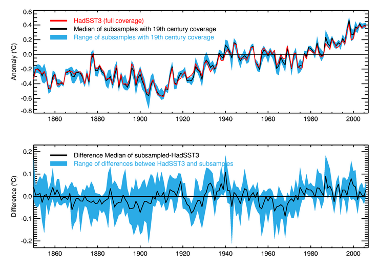
The HadSST3 coverage uncertainty is largest (with a 2-sigma uncertainty of around 0.15°C) in the 1860s when coverage is poorest. This falls to 0.03°C by 2006. That this uncertainty should be so small – particularly in the nineteenth century – is surprising. To an extent the relatively small uncertainty might simply be a reflection of the assumptions made in the analyses used by Kennedy et al. (2011b) to estimate the coverage uncertainty. Another way of assessing the coverage uncertainty is to look at the effect of reducing the coverage of well-sampled periods to that of the less well sampled nineteenth century and recomputing the global average.
This figure shows the range of global annual average SSTs obtained by reducing each year to the coverage of years in the nineteenth century. So, for example, the range indicated by the blue area in the upper panel for 2006 shows the range of global annual averages obtained by reducing the coverage of 2006 successively to be at least as bad as 1850, 1851, 1852 and so on to 1899. The red line shows the global average SST anomaly from data that has not been reduced in coverage. For most years the difference between the subsampled and more fully sampled data is smaller than 0.15°C and the largest deviations are smaller than 0.2°C. For the coverage uncertainty on the global average to be significantly larger would require the variability in the nineteenth century data gaps to be much larger than in the well observed period.
The structural uncertainties associated with estimating SSTs in data voids and at data sparse times are somewhat better explored. A variety of different statistical techniques have been applied to both the in situ and satellite data providing a range of sometimes quite different results. The problem of creating globally complete analyses is challenging because of the relative sparseness of early observations, the non-stationarity of the changing climate and the fact that more observations are missing at colder periods than at warmer ones.
One particular concern is that patterns of variability in the modern era – which are used to train the statistical models – might not faithfully represent variability at earlier times. It is not clear to what extent this question has been resolved. Smith et al. (2008) allow for a non-stationary low frequency component in their analysis which weakens the criticism as it pertains to this analysis. They used sub-sampled climate models to optimise their algorithms in periods when data are few. Ilin and Kaplan (2009) and Luttinen and Ilin (2009) used iterative algorithms that make use of data throughout the record to estimate the covariance structures and other parameters of their statistical models. However, such methods will still tend to give a greater weight to periods with more plentiful observations.
Another concern is that methods which use Empirical Orthogonal Functions to describe the variability might inadvertantly impose long-range teleconnections that do not exist in the data (Dommenget 2007). Smith et al. (2008) explicily limit the range across which teleconnections can occur, likely mitigating this problem. A number of analysis methods have a tendency to lose variance at a range of time scales either because they do not explicitly resolve small scale processes (Kaplan et al. 1997, Smith et al. 2008) or because in the absence of data the method tends towards the climatological average (Ishii et al. 2005). Rayner et al. (2003) used the method of Kaplan et al. (1997) but with certain changes to the method to explicitly resolve the long-term trend and improve small scale variability where observations were plentiful. Karspeck et al (submitted) analyse the residual difference between the observations and the Kaplan et al. (1997) analysis using local non-stationary covariances and then draw a range of samples from the analysis posterior distribution in order to provide consistent variance at all times and locations.
Yasunaka and Hanawa (2011) examined a range of climate indices based on seven different SST products. They found that the disagreement between data sets was marked before 1880, and that the trends in large scale averages and indices tend to diverge outside of the common climatology period. For the global average, the differences between analyses was around 0.2K before 1920 and around 0.1-0.2K in the modern period. Even for relatively well observed events such as the 1925/26 El Nino, the detailed evolution of the event varied from analysis to analysis. The reasons for the differences are not completely clear because each data set is based on a slightly different set of observations, which have been quality controlled, and processed in different ways.
Currently, only a few groups provide explicit uncertainty estimates based on their analysis techniques. As noted above, the uncertainty estimates derived from a particular analysis will tend to underestimate the true uncertainty because they are conditional on the analysis method being correct.
JC’s assessment
In the 6 hours that I have been able to devote to this, here is my first take on their uncertainty analysis.
This effort represents a substantially more sophisticated assessment of the uncertainty than was seen in HADSST2 (which was the basis for much of the IPCC AR4 analysis). The have clearly identified the primary uncertainty locations, while at the same time allowing for the possibility of unknown unknowns. The statistical sophistication of the error analysis is also substantially improved. The acknowledge the incompleteness of their uncertainty quantification, i.e. there are some sources of uncertainty that were not quantified and they acknowledge that other methods may produce different uncertainty values.
My main critique of their uncertainty analysis is the issue of structural uncertainty and specifically their estimate of the uncertainty associated with incomplete coverage. Sophisticated statistical techniques (e.g. EOFs) are used to fill in missing data, using relationships and variability derived primarily during the period of good data coverage in the latter half of the 20th century. The farther back in time you go prior to this period, there is generally reduced global coverage of observations, with coverage very low prior to 1920 over much of the global ocean. So basically, values over much of the global ocean prior to 1950 are determined from a statistical model.
Errors associated with using this statistical model to determine the global average time series is estimated by subsampling the observations (primarily ship tracks) in the earlier period against reanalysis data for the modern period. One study has used simulation results from the GFDL model to assess the error. The coverage uncertaingy identified for HADSST3 (global annual average) has a maximum value of 0.08C (1-sigma) and 0.15C (2-sigma) circa the 1860’s. These value seems implausibly low for periods when data for a large portion of the global ocean is created by a statistical model.
A more sophisticated and systematic analysis of different assumptions about climate variability prior to the mid 20th century and different statistical methods is needed to provide a more realistic estimate of the coverage uncertainty. This might be accomplished by using coupled climate model simulations for the models that more reliably simulate the ocean climate for the last 20th century that each have multiple ensemble members to test the various statistical assumptions and subsampling on different realizations of the ocean climate since 1950.
The other structural uncertainty issue is the actual method for combining different biases and the uncertainty model itself. In the context of parametric uncertainty for the bias corrections, the determination of uncertainty is associated with a number of underlying assumptions that are uncertain in themselves.
The HADSST group are to be commended for their extensive efforts in attempting to quantify uncertainty in the HADSST3 dataset. They admit that their analysis is incomplete. I suspect that the major source of unaccounted uncertainty is structural error in their method for dealing with incomplete coverage. Improved methods to analyze uncertainty in the SST data set, particularly that accounts for structural uncertainty, are needed to provide a better understanding of the global SST and to produce more realistic assessments in the IPCC.
Here are two excerpts from the uncertainty web page regarding their advice on using the data set:
Finally, the work of identifying and quantifiying uncertainties will be pointless, if those uncertainties are not used when the SST data sets are used. Uncertainty estimates provided with data sets have sometimes been difficult to use, or easy to use inappropriately. As pointed out by Rayner et al. (2010), “more reliable and user-friendly representations of uncertainty should be provided” in order to encourage their widespread and effective use. HadSST3 has been produced as a set of interchangeable realisations that together define the bias uncertainty range of HadSST3. It is hoped that providing these 100 realisations in a form identical to the median estimate will encourage users to explore the sensitivity of their analysis to observational uncertainty with little extra effort. It is also suggested that users run their analysis on a range of different SST analyses.
It is common in detection and attribution studies only to use data where there are observations by reducing the coverage of the models to match that of the data. This reduces the exposure of the study to structural uncertainties associated with analysis techniques.
Let’s see if the IPCC AR5 adopts this advice in their assessments of likelihoods and confidence levels associated with the surface temperature record.
And finally, getting back to Sharper00’s challenge, Figure 11 of Part 2 clearly shows uncertainties exceeding 0.3C in the 19th century. And the authors admit that their uncertainty analysis is incomplete and likely to be too low:
As noted above, the uncertainty estimates derived from a particular analysis will tend to underestimate the true uncertainty because they are conditional on the analysis method being correct.

I’ll say again …
Lindzen, Spencer, and some others catch a lot of heat for attempts to verify climate models by some of the more modern, more accurate measures, but I believe they are moving in the right direction. Temperature, CO2, or precipitations reconstructions have many issues that are well known. But modern instrumentation is making possible characterizations of the climate system that were heretofore impossible.]
The comparison of the temperature profile of the atmosphere to that predicted by climate models is a good effort, and the climate models have come up short. Now we are getting heat and temperature profiles for the oceans. Those can be compared to predictions of climate models as Spencer has attempted.
Even the Lindzen and Choi paper can be useful to validate climate models. This, in spite of shortcomings in the methodology WRT the determination of Earths climate sensitivity. Data from the climate models can be processed the same as in the paper. The major forcing/response timings found by L&C should be the same for a successful model. The limited sensitivity determined by L&C should be the same in a successful model.
Using modern measurements of air temperature, incoming/outgoing radiation, and ocean temperature/heat content should provide much more robust techniques of climate model validation.
“And finally, getting back to Sharper00′s challenge, Figure 11 of Part 2 clearly shows uncertainties exceeding 0.3C in the 19th century. And the authors admit that their uncertainty analysis is incomplete and likely to be too low:”
You’re not really saying you’re going to add quotes around experts for working scientists at CRU because you eyeballed a slightly different number of a graph are you?
What do you consider to be the “true” uncertainty range. You’ve certainly expanded on your previous comments but along the same lines – here’s a list of problems with the data [therefore] the number must be different to 0.3. I don’t see anything to suggest that the 0.3 number doesn’t already include the problems you’re listing and I (still) have no idea how far off you think the range is.
Ideally you’d show that people at CRU produce much lower uncertainty ranges than experts elsewhere if you absolutely insist on going after those people. Even more ideally though you’d show the range of uncertainties that exist in the literature so that I, and everyone else, gets some idea of what the field in totality thinks of uncertainty in those temperatures.
If your preferred number is quite different to that of any published expert you’d need to explain why that is, hopefully minus the terms “climategate” and/or “conspiracy”.
Sharper00 you actually have to read the stuff i posted. They state the uncertainty estimates are greater than for HADSST2 (used in IPCC AR4). They then list a number of uncertainties that were not quantified, that would increase the total uncertainty. my point is that the uncertainty has not yet been adequately quantified for the reasons stated in the article, the web site, and my comments.
I read your quoted excerpts and your comments, I haven’t read the linked papers except to check the figure you mentioned.
Why are you so evasive about what the number should be? Are we talking about 0.6? 1 degree? 10 degrees? I have literally no idea how far off you think they are.
Saint Judith writes “My point is that the uncertainty has not yet been adequately quantified.” So, what part of that do you not understand? She said that the uncertainty has not been adequately quantified. That means that there is no number that can be presented as the uncertainty. So, your persistent question about the specific number is bratish, at best. As she explains, there are unknown uncertainties that would increase the uncertainty beyond .3, so the .3 number is too small. What about this do you not understand?
Theo,
It seems a fair question to me. Judith can only know if the figure of 0.3 is significantly too small if she has at least some notion of what the true figure should be.
Another question would be if Judith thinks the measured temperatures are likely to be under or overstated.
well that is the point about uncertainty, we have no idea if the real temperatures and trends are higher or lower
I suppose you could use ramesdorf’s semi empircal sea level/temperature model.
If you had a good estimate of sea level you could use that model to put a limit ( perhaps) on the size of the uncertainty by . nothing wrongworking from the estaimte of sea level to the estimate of temperature.. might give you pretty wide error bars.. hmm its late and now I have to go get hadsst3 data..
I don’t know what you’ll do for uncertainty, but at the very least you’ll establish the Outer Banks of global temperature for the last 2,100 years.
We can guess reasonably well. Which way did the IPCC AR4 writers and their bosses WANT the trends to go? Odds are approaching certainty that that’s the way the biases have gone. Systemic bias doesn’t pick a direction at random, notwithstanding any and all formal assumptions to the contrary.
Well, Judith that’s not strictly speaking true. You could say N degC +/- 0.15 deg C. Or its just as valid to say N deg C +0.1 /-0.2 deg C if you had reason to believe there could be a negative systematic bias. But that’s just a minor quibble.
I, too, hope the Berkely group get the chance to tackle the this. If they do, people like Fred, Sharperoo and myself would, I’m sure, accept their findings whichever way it goes. But do you think any new study will make a jot of difference to the vast majority of skeptics/deniers on this blog? They like the phrase ‘we simply don’t know’ and neither you, I nor the Berkely Earth group are likely to shift them away from that.
Here is what the Berkely group needs to tackle:
http://chiefio.wordpress.com/2011/07/01/intrinsic-extrinsic-intensive-extensive/
whether what is being used is a meaningful metric, not just whether the adjustments (which they apparently are NOT verifying) are appropriate and the computations are reasonable
Chiefio’s post is really interesting. I will try to wrap my head around this one and do a post on it next week.
Judith
Well put by Chiefio.
Similarly, see Roger Pielke Sr. posts on “Global Average Surface Temperature”
Especially:
Climate Science Myths And Misconceptions – Post #1 On The Global Annual Average Surface Temperature Trend
Climate Science Myths And Misconceptions – Post #2 On The Metric Of Global Warming
As far as I can see, it has been a common knowledge that average surface temperature is in not an ideal parameter to describe warming of the earth. The total energy of the Earth system is in principle much better and the average temperature is just a proxy of that.
There are numerous issues related to the average surface temperature. In connection of SST one good example is the change in area of sea ice. As long as we have open sea the temperature of the surface remains certainly close to 0 C or above, but when we have ice and snow cover, the surface temperature of snow may easily be much lower. The change in the heat balance of Earth is in such case much less than the change in the average surface temperature.
All this is true, but so what? We knew already that the average surface temperature is only a proxy. It’s used because determining the extensive variable the total energy of the Earth is too difficult even excluding the interior of the Earth and absolute values and concentrating in the variations in the energy content of the atmosphere, oceans and continental areas to a depth of a few meters.
That the average temperature is a deficient proxy tells that even it is not a perfect parameter to describe warming of the Earth system, but up to now it’s one of the best parameters. How dangerous the warming is, is not at all dependent on the quality of the parameters that we have to describe it. If it’s dangerous, it is whether we have a good parameter or not, and vice versa.
Pekka Pirila,
“How dangerous the warming is, is not at all dependent on the quality of the parameters that we have to describe it. If it’s dangerous, it is whether we have a good parameter or not, and vice versa.”
That is a true statement, but not very helpful. The only way we can know “how dangerous the warming is,” is through those “parameters.” So, while the issue of whether they are “good parameter[s] or not” does not impact how dangerous the warming is, the reliability and accuracy of the parameters has everything to do with the policy decisions being urged.
There are many kinds of uncertainties. Listing them is of no help, if the risk is real, and the more we have uncertainties the more possible it is that the consequences will be severe. This is true as long as the uncertainties are symmetrical as they are in this case. Only, when we can reduce the uncertainties asymmetrically from the side of higher risks, can we feel more safe with reduced uncertainties.
“It seems a fair question to me. Judith can only know if the figure of 0.3 is significantly too small if she has at least some notion of what the true figure should be.”
This is one of the most common, and hilariously inane, memes of the CAGW tribe. You can’t say our made up figures are wrong if you don’t substitute your own made up figures. Brilliant. It is of course just another iteration of the “shifting the burden of proof” trope also so popular with climate progressives.
I don’t have to know the global average temperature of the Earth in 1422 to know that Michael Mann cannot determine that number within a tenth of a degree based on an extremely limited number of proxies. I don’t have to go out and measure the temperature in thousands of locations in the Antarctic to know Eric Steig’s claims to statistically determine those temperatures with similar precision in grid squares with no thermometer within a thousand miles is fantasy. I don’t have to know the global average sea surface temperatures of 100 years ago within 5 tenths of a degree to know that consensus scientists don’t know that figure within 3 tenths of a degree. I wonder if any of the commenters urging this “logic” even believe it themselves. I hope not.
Manufactured data cannot be magically changed into real data by statistical analysis. Data with potential errors of 2 or 3 degrees when collected cannot be massaged to give an average that is accurate on a global scale to tenths of a degree. You either have the data or you don’t. Either deal with the limitations of what is available, or kindly shut the hell up. Hubris is not the same as knowledge.
We don’t know what the global average sea surface temperature was 100 years ago within tenths of a degree. No amount of waving of hands and stamping of feet is going to change that. You CAGWers can believe whatever you like. The rest of us will live, and vote, in the real world.
I agree, GaryM.
That is an old trick of propaganda artists:
Just ask your critics to explain quantitatively the correct value for a number that you got caught reporting without justification.
With kind regards,
Oliver K. Manuel
GaryM,
I agree with you about the use of statistics to fill in gaps in the data. However, there are many scientists who are not “CAGW”. It is important to send up satellites to obtain data with which to monitor the earth’s environment. Unfortunately, funding for this is dependent on there being a “crisis” and there does not seem to be any other way of motivating people.
Rose
GaryM,
“Data with potential errors of 2 or 3 degrees when collected cannot be massaged to give an average that is accurate on a global scale to tenths of a degree”
This might seem a reasonable enough comment to many people, but its just not true.
For instance, say, 19th century thermometers were only accurate to +/- 5%. (They actually were much better than this!)
So, when measuring an actual temperature of 100degF any result in the range 95 degF to 105 degF would have been possible depending on the particular thermometer chosen.
In the 19th century there would have been many thousands of readings taken with hundreds of different thermometers. But say we just looked at one reading per thermometer, taken with 100 different thermometers which are then averaged out. How close would our 19th century mariners have been to 100 degF?
I set this up on a spread sheet to simulate the process and in 10 runs measured:
99.9,100.1,100.3,100.5, 100.1,100.5, 99.8,99.7.100.0,98.8
So the standard deviation would be about 0.3 and the worst case 0.5 degF error.
And yet any one reading was only known to within 5 degF !
This is just a very simple and easy to understand statistical analysis – nowhere near the level of sophistication that Judith Curry was writing about. But, nevertheless it does show that meaningful results can be extracted from very ‘noisy’ data if the correct statistical procedures are applied.
I think you are confusing the problem of calculating the error when the mariner takes 10 measurements at 100 locations at the same time (and estimates the average at that point in time), and making the same estimate when only 1 measurement is taken on that day at each location, and some of the locations were missed, and some measurements occured at 6.00, and some at 8.00.
“confusing the problem” No
Simplifying to illustrate a point. – Yes
tempterrain,
“So, when measuring an actual temperature of 100degF any result in the range 95 degF to 105 degF would have been possible depending on the particular thermometer chosen.”
First, the fact that you can find the standard deviation in a defined set of numbers, given a starting “actual temperature,” and a given range of error, has nothing to do with trying to find the actual temperature and standard deviation from a set of numbers for which you don’t even know what the actual potential error range is.
By establishing the “actual temperature” as 100, and defining the error range as +/- 5%, you gamed the problem. Are you surprised that, having defined the starting point, and the error range, you can determine a standard deviation for a set of numbers generated on that basis? How is that analogous to taking a set of numbers, and from them determining both the “actual temperature,” and the range of error? You can find the mean of any set of numbers, but that begs the question of whether the mean equates to “actual temperature,” which it assuredly does not.
It also misses the fact that the measurements are in different locations, on different dates, with different weather conditions. Assume the accuracy of each thermometer is +/- 5% (this is climate science, we can assume lots of things), you also have to factor in at least the time of day, day of the year, and depth of the water measured (we are after all talking about global average temperatures). Each of these factors must nevertheless influence the temperature reading and introduce their own potential errors.
Then there is the issue of the global scope of the measurements, and paucity of sites from which measurements were taken.
The fact that you can find the standard deviation of a set of non-random numbers doesn’t tell you anything helpful when it comes to measuring actual temperature within tenths of a degree from historical data based on antiquated equipment with little control over the method of collection and huge gaps in the areas measured.
Your comment is a classic example of the faulty logic that seems to permeate climate science. Finding the standard deviation, which seems so mathematically precise, masks the assumptions you have to make to get there.
Tempterrain,
I have to call you on this one. This is a common misunderstanding with people outside the instrumentation field. One degree Celsius change in temperature is not a 1% change. Zero temperature is -273.15 degrees Celsius. That one degree change is actually approximately 0.35% change. This gets even more difficult a concept for folks that use the Fahrenheit scale where zero is -459.67 degrees. Each Fahrenheit degree is about 0.19%.
As for the ‘correct’ statistical method being able to extract more accurate results from noisy data, that only applies if the signal you are attempting to find is repetitive over several cycles in the sample time frame and the data noise is external to measurement method. That works great for digging radio signals out noise. It is a grand stretch to claim you can do the same for a linear or nearly linear change over that time frame.
An assumption that averaging many crappy temperature readings will provide a more accurate temperature measurement is simply bogus. The assumptions behind this are many and false. As a trivial example, averaging many readings from a thermometer that reads one degree high will provide a number that converges on one degree high. Though trivial, the problem this example describes extends to all past temperature readings.
Measurement instrument errors, measurement method errors, and recording problems must all be assumed to cancel each other out for the assumption of random errors to be true. The point is that it is an ASSUMPTION not proven out in the field of instrumentation design and implementation. The volume of text available discussing instrumentation and instrument data usage far outweighs all of the material produced by climate scientists to date.
If you have a set of measurements Mi each of which is a sum of the true temperature at the point of the measurement Ti and an error Ei. The average of n observations is
(M1+M2+M3+…Mn)/n
which is
(T1+T2+T3+…Tn)/n + (E1+E2+E3+..En)/n
The first term is the average of the temperatures at those n locations and times. The second term is the sum of the errors in those measurements. Now depending on how those Errors behave you can get all sorts of different effects.
If all the Es are simple independent uncorrelated gaussian noise then the average of a large number of them will tend to zero so the average of the Ms would tend towards the average of the true temperatures (Ts) as n increased.
If all the E’s are equal to 1K then the average will be 1K. We don’t improve the situation by averaging at all.
So in this strange argument everyone is making different assumptions about the E’s and how they behave. For real SST measurements some of the errors will be of the nice kind that obligingly diminish when averaged. Others won’t.
One thing that we can notice from the above formulas is that there is no basis for this claim:
“As for the ‘correct’ statistical method being able to extract more accurate results from noisy data, that only applies if the signal you are attempting to find is repetitive over several cycles in the sample time frame and the data noise is external to measurement method. “
Whether the errors cancel or not has nothing to do with repetition over several cycles.
If the errors are uncorrelated and of the same order of magnitude they will cancel to a significant degree, and the accuracy of the final result will improve proportionally to the inverse square root of the number of observations. Unfortunately the errors are certainly not totally uncorrelated, and that rule will apply only to the uncorrelated part of the errors. (In addition the relative weights of the observations vary, and this adds an additional factor to the resulting estimate of the uncertainty from uncorrelated part of the errors.)
Pekka,
“Whether the errors cancel or not has nothing to do with repetition over several cycles.”
Actually, not true. Without repetition, your signal cannot be distinguished from systematic error. You can only speculate that a linear trend is significant, not assure that it is.
GaryW,
You’re right to point out that I should have said “For instance, say, 19th century thermometers were only accurate to +/- 5deg F” not +/- 5% as I originally wrote. But apart from that what I said was correct.
You’re right to when you say “averaging many readings from a thermometer that reads one degree high will provide a number that converges on one degree high” That’s known as systemic error. And if all 19th century SST readings were taken using the same thermometer you’d have had a point.
GaryM,
You mention ” standard deviation of a set of non-random numbers ” The numbers were generated on a spreadsheet using Excel’s random number generator so they the net result was what, in electronic terms, I would say was real data (signal) and unwanted randomness (noise). Separating the two is a standard requirement in everyday telecomms.
You are keen to point out that my simple example ” also misses the fact that the measurements are in different locations, on different dates, with different weather conditions.” Well, I could send you my spreadsheet if you like and you can start to add different these factors one at a time to increase its complexity. If you do it all properly, you will still find that it is possible to make sense of a mass of data which looks at first glance to be so riddled with errors that the task is hopeless. If Judith’s suggestion of giving the task to Berkely’s Earth group ever comes about, that’s what they’ll be doing, but with a lot more sophistication than I’m capable of demonstrating. Ask her if you don’t believe me.
“Actually, not true. Without repetition, your signal cannot be distinguished from systematic error. You can only speculate that a linear trend is significant, not assure that it is.”
Even with repitition the signal might be indistinguishable from the systematic errors. In that case, you need information about how the measurements were made and try to work out the systematic errors that way.
Neb,
“Even with repitition the signal might be indistinguishable from the systematic errors. In that case, you need information about how the measurements were made and try to work out the systematic errors that way.”
Yes, true. There in is the problem. We are dealing with data from measurements taken in a number of incompatible ways and then assuming we can correct for it. None of this correction is field verified, merely statistically tweaked. In the case of linear trends, even if we were to assume systemic errors are zero, we run into the problem that what we may be observing my be simply a segment of a longer period repetitive signal or simply low frequency noise. Even if that trend meets our expectation, it may be false.
Of course, the point I am trying to make is not that a trend may not exist, only that the existing historic temperature data cannot be massage to produce accuracy values better than a degree or two Celsius. Even that assumes we will gain a better understanding of error sources. Sticking a tenth of a degree fraction on the end is false advertising.
Gary,
Whether there is or is not cancellation of certain errors depends only on the properties of the errors and not at all on the properties of the real phenomenon. Knowing something about the real phenomenon helps in determining, what the errors in individual measurements are like. Knowing that the phenomenon is periodic, is one example of such helpful knowledge, but certainly not the only way of justifying some assumptions about the errors.
Uncorrelated errors are always present and they do always cancel according to the same rule, but what is not known a priori is their size or the size and properties of systematic and correlated errors.
A number of people have pointed out the importance of separating the random and systematic components of the uncertainty. The random component will certainly be an important contribution to the uncertainty if we want to know what the SST was at a particular point on a particular day, but it will be less important if we’re looking at the trend in global average temperature.
The measurements from most ships will have some kind of systematic bias, but this will not be exactly the same for all ships, so some component of that will be reduced by averaging the measurements from many ships together. All of which leaves the pervasive systematic biases affecting large numbers of observations.
The pervasive systematic errors are most important at longer time scales. If we had no other information about the measurements a good rule of thumb might be to allow for a systematic error of a degree or two. Much more than that and the mariners might have been better advised to stick their thumb in the water rather than a thermometer.
However, there is a long literature on the sizes of systematic errors in SST measurements going back to papers published in the early 20th Century. Generally the sizes of the systematic errors were found to be a few tenths of a degree rather than 1.0K or more. The largest pervasive systematic errors identified – around 0.5K – come from measurements made using canvas buckets.
For a review of these effects see:
http://www.knmi.nl/~koek/Publicaties/10.1002_wcc.55.pdf
There is a table summarising estimates of engine room measurement biases in part 2 of our paper which can be obtained here:
http://www.metoffice.gov.uk/hadobs/hadsst3/
John Kennedy
Well put re:
For some “home science” exploring our Sense of Touch
The real fun begins in: Assessing skin sensitivity – temperature receptors
GaryM – spot on. Top rule in communications – never do numbers.
It would seem to imply an opinion on what the true figure should be or at least something in the ballpark. I doubt the opinion would be that the true figure could be anything.
Incorrect. You can tell quite quickly if the error limits are too low simply by the variation in the data (sd/cv’s) and the amount of parsed, or missing data.
The (fully understandable) use of models to fill in data blanks precludes a .3 error limit. I’ll have a detailed look at the analysis later today to see what i can come up with (as this sort of thing is more my area), but from first pass i agree that .3 is optomistic.
HOwever- they were STILL right to quote that figure if thats what they’ve calculated- especially as they’ve qualified it by stating themselves that their analysis is incomplete and probably too low.
Now you are writing about significance. She said that the uncertainty has not been quantified. What is the significance of the unquantified?
Good stuff Judith. It’s good that you’re looking so closely at the huge uncertainties that surround such an important part of the climate change narrative.
I would place the uncertainties in the global surface temperature at around 1C ( I have problems with the notion of ‘global’ as well)
The SST record prior to 1950 is so vague that I would hesitate to place any figure on it, as so much of the material used is unreliable. Care to quantify it?
tonyb
Wrestling with uncertainty in this data set is a huge job. I hope the Berkeley Earth group gets funded to tackle this issue.
1 sigma +-1C.
Gosh at -2.4C in 1850 we have a huge global warming problem.
you don’t get to pick just one side of the uncertainty.
Mosh
Would YOU care to put a considered figure on it?Are you happy with 0.3?
Tony
.3 is too narrow, 1C is too large. But throwing numbers out without a clear method isnt really helpful. Still reading their paper..
You answer his question (quite clearly) and ‘you absolutely insist on going after those people.’ Then he turns it around, ignores what your original assertion was and accuses you of being ‘evasive’ because you can’t make more precise (than a less than/greater than) estimate based on what you (based on the literature above) established to be insufficient information to nail down the .3 degree uncertainty estimate.
Did i get that right? It’s hard to be certain given the impression that reason only exists on one side of this.
Great explanation and discussion point for those that are open to it, though. Thanks
I was a little puzzled by the ‘you absolutely insist on going after those people’ quote myself. Seems a bit defensive.
I found the implication that the researchers that produced the 0.3 number were not just of a contrary opinion but not deserving of the descriptor “expert” bizarre and itself in need of justification.
You don’t need anything else sharperoo. Judith has fully justified her earlier statement regarding uncertainties. You are wriggling by trying to introduce distractions. Time to back down fella as you are starting to make a fool of yourself.
RobB,
It looks to me that you are claiming victory on this one. A clear example of Danth’s Law. “If you have to insist that you’ve won an internet argument, you’ve probably lost badly.”
http://www.telegraph.co.uk/technology/news/6408927/Internet-rules-and-laws-the-top-10-from-Godwin-to-Poe.html
Or you are arguing with a leftist who will never admit fault.
Maybe I missed it… but it seems to me that a key factor in the early period was the ‘human instrument’ reading those early thermometers. How did the quality of those readings compare in some gale force storm versus a nice calm day? I find it almost hilarious when I see such exact figures from such an inexact process.
That said, I have no doubt that there was warming since then as the Little Ice Age was ending. As far as I can tell, it still is… pending what the Sun does next.
“Sharper00 you actually have to read the stuff i posted.”
But that’s so painful, which is a good part of the problem right there.
Well it is much easier to read my post than it is to read the two journal articles plus additional articles that it referenced, plus the extensive documentation on their web site.
Have YOU read them pokerguy? If so what’s your opinion of Dr Curry’s analysis? If not, why not?
” Figure 11 of Part 2 clearly shows uncertainties exceeding 0.3C in the 19th century. And the authors admit that their uncertainty analysis is incomplete and likely to be too low”
Judy – Figure 11 illustrates the principle that the uncertainties that are critical depend on the question being asked. If we have inadequate sampling, and short time intervals, the statistical uncertainties from random fluctuations and random measurement errors can be large, but would tend to cancel out as the number of observations and length of time increases. In the case of systematic biases (e.g., a technique that consistently overestimates or underestimates temperature), additional measurements will not cancel the effect. Here, however, the error will be in the absolute values of temperature, which may or may not be the subject of greatest interest.
In many cases, what is of particular interest are the anomalies – the changes over time relative to a baseline. With sufficient time, the random fluctuations are likely to cancel, and systematic biases will not affect the anomaly calculations unless the biases change with time.
This has undoubtedly happened in some cases, but for Figure 11, I get the sense that the trend in anomalies, if analyzed statistically, will be characterized by variances of less than 0.3C. That is most likely after 1910, when a century long SST warming emerges from the data, but I’m not sure it isn’t also true for the earlier data. On the other hand, at individual times, 19th century uncertainties certainly appear often to exceed 0.3C.
sharper00’s guide to learning about something he doesn’t currently know about:
-Firstly I determine whether the specific topic represents basic, intermediate, advanced, expert or cutting edge knowledge. The first two are often readily available on the internet, the rest may require access to text books or journal articles. The last two will often be subject to disagreement among among experts. I would classify a topic like “Uncertainty in historical sea surface temperatures” as cutting edge requiring access to recently published primary scientific literature.
-Secondly I evaluate the range of opinion that exists among experts and researchers, to what degree parts of the range are supported and possibly the main points which separate groups of experts. This is in order to understand why the range exists in the first place and what represents a spectrum of supportable opinion. On this topic I am still completely unclear what the uncertainty range is except that some people have produced a number that others dislike.
-Thirdly I determine where the specific proposal sits in relation to that range. Is it within the range? Is it outside it? Is it far outside it? I haven’t yet seen anything to evaluate for this topic even if I had the answer from step two. Possibly Dr Curry is siding with a group of experts, possibly she’s outside the range produced by all experts. I have no idea.
None of this means the experts are necessarily right or wrong. I consider it absolutely critical to first know and understand what they’re saying before discarding it however. I consider it a huge red flag that people who oppose basic science like the greenhouse properties of carbon dioxide are unable to explain how it’s supposed to work (they instead declare it cannot work) or how experts could come to think it would work.
This is the mode of investigation I use. I don’t immediately delve into published primary literature to see to what degree they appear to confirm or reject a specific proposal. I consider this a waste of time without a wider understanding of the field.
Fourthly, how much time do you believe would be necessary to determine the uncertainty in subject dataset?
Uncertainty is just another property of the dataset, I have no explicit step for it anymore than I have for “Determine what year the dataset starts”
If there’s disagreement around the uncertainty all the other steps apply. Making a direct judgement on uncertainty would in most cases involve me getting a couple of new degrees and working in the given field for years. I can only do that so many times.
So you concur that 6 hours is not enough time.
I would expect someone that is already an expert (i.e. Dr Curry) to be aware of the factors involved. If 6 hours is going to be spent explaining it I’d prefer it to be in the form of “Here’s an overview of who thinks what and why” rather than “Here’s some papers that think uncertainty is wrong too, go read them everyone”
You come off sounding hostile and bitter. I appreciate the time Dr. Curry spends on the blog – I’m sure you can take your own medicine and do the analysis. You may have more time on your hands than she.
Are you under the impression that Professor Curry owes you something? How much did you pay her for this course?
Excellent post. It should surprise no one that efforts to accurately calculate uncertainty, as well as efforts to mitigate potential sources of error and bias that contribute to uncertainty, are ongoing among the scientists working on SST estimates. It’s good to see that work moving forward, and I’m excited to see how the AR5 benefits from the work of the last five years.
Thanks for clarifying your reasoning. By considering only the level of agreement among experts, you ignore the key element of assessing the amount of evidence available upon which to base a judgment. By reading the primary literature and assessing the methodologies used, I conclude that the uncertainty estimates are too low. And the authors of this piece do not disagree with me. I can make such an assessment of the uncertainty being too low without myself actually producing my own estimate. This is called a critique, or an assessment.
“By considering only the level of agreement among experts, you ignore the key element of assessing the amount of evidence available upon which to base a judgment”
As I stated, it’s where I first start. When the proposal is understood relative to the actual topic it’s being made I can start to evaluate it in detail, presuming I deemed it interesting or noteworthy enough to merit it.
You yourself invoked the experts by quote quoting the ones at CRU – a clear insinuation that their number was so very wrong they didn’t deserve to be called experts at all.
“By reading the primary literature and assessing the methodologies used, I conclude that the uncertainty estimates are too low.”
Which is nice but in order to evaluate your opinion more information is needed. Like, for example,how low you think it is and who else might support that amount of difference (not simply any difference).
“I can make such an assessment of the uncertainty being too low without myself actually producing my own estimate.”
You don’t have to produce your own estimate (it would be nice) but you do have to say how wrong the estimate your critiquing is, to some degree of approximation, or else it’s a pretty poor critique.
It does seem that if you think the uncertainty estimates are too low, you must have some notion of what is a more appropriate estimate.
A bigger number
Exactly. if there are six sources of uncertainty and one is estimated to be 0.3 degrees then the total is larger. One does not have to have an estimate of the total to know this
Yeah – I figured that’d be your answer.
So I gather that you have no idea how much more uncertainty there is. It could be bigger by a factor of .001, .001, .01, .1, 1,100, or 1,000,000. But you are nonetheless pretty certain it is higher than the estimate.
Somehow I could have guessed that before you did all that work. In fact, I’d say that any reader of your blog could have guessed that before you did all that work.
Kind of makes me wonder why you bothered.
Looking at the Figure 11, the typical total estimated 2-sigma uncertainty for the period 1850-70 is about 0.2 degrees from the best estimate. The statements made in the paper indicate that it’s authors consider it quite possible that this is an underestimate. They don’t say, how much larger the uncertainty could be, but adding 50% to the estimate might be a reasonable guess. Thus the total 2-sigma uncertainty would be about 0.3 C.
Estimates of uncertainty of that whole period beyond 0.3 C would in my view be contrary to the implications of the paper although they have not been explicitly excluded.
Nature provides the paradox ie the singularity that tests both the observations and the theory a binary problem,eg Krakatau here either the observations are incorrect or the physics.
curryja, you need to bear in mind that the uncertainties tend to add in quadrature so a new source of uncertainty would need to be quite hefty – relatively speaking – to show a noticeable increase on what’s already there.
You and sharperoo are confusing the math of uncertainties with judgements of the phyisclal evidence that the math represents. Professor Curry is talking about the latter not the former.
I’m well aware of the difference.
There is no reason why the incomplete coverage (?) uncertainty can’t be quantified. Our host even suggested a couple of ways at coming at it. If it were quantified then what I said would be the case.
What curryja offered us was a hunch – a well-founded one as it turned out. The hunch was that the uncertainty estimates are too small in the nineteenth century and suggested that this was due to incomplete coverage uncertainties being underplayed.
Fair enough, but finally what we need is to attach a number to it. No one thinks that the uncertainty is 10K, some here have gone for around 1K as a ball park figure for the total uncertainty. We can debate the pros and cons of various estimates, but first someone needs to put forward a reasoned estimate.
One need not confirm the precise depth of water they are in to establish they are in over their head.
The authors above say, too low. Judith says ‘too low’.
I’m guessing you mean “Fair enough, but finally what science needs is to attach a number to it.”
That should be interesting. Could be difficult given the conditions/unknowns that Judith and the cited material highlights.
“…but finally what we need is to attach a number to it.”
That, in a nutshell, is what is wrong with the consensus climate science. “We need to attach a number to it.” If I were a scientist, my position would be, we need to find out if we can attach a number to it. We “need” to know what the historical global average temperature was within tenths of a degree. Rather than, what do we actually know about the historical global annual temperature.
The “need” is solely driven by politics. It is this thought process that skeptics decry, and CAGW advocates do not even recognize.
“Quadrature”? “Tend to”? What in the world are you talking about? Is this tendency physical or mathematical? It sounds Aristotelian.
I can only relate the remark about errors not being strictly additive to my experience in the elctronics field, mainly tracking radars. In addition, I am writing from a technician point of view, not an engineer. (In other words, please cut me some slack if I get way off base, just point out my mistakes and correct them)
What is typically seen there is that an error budget is derived from many factors (some are glint, mislevel, coning, difference between physical and RF pointing angles) In most cases, the total error budget is comprised mainly of one or two factors.For the purposes of this discussion, I will use the following case of determining angular tracking error of a radar.
A siimple method, and one that is used estensively in my line of work, is to calculate the RMS track error (take the square root of the sum of the squares of mean error and standard deviation). In this method, if you have 1 degree mean error and 1 degree standard deviation, the final result is not 2 degrees (simple sum), but 1.41414 degrees. j other words the end result resembles a vector, with the answer being the distance between the endpoints of each individual vector.
I hope this helps, or at least makes sense…
Rick,
Good point. Out of phase errors do not always add linearly. Of course, if they are random with respect to each other they can in some time intervals add linearly. Of course, what we are interested here is in how this relates to sea temperature readings from about a century and a half ago.
Looking at your statement about out of phase signals not adding linearly another way, whatever the source or magnitude of non-correlated noise, it will always add to the total error. It simply may not be a linear addition.
“Have YOU read them pokerguy? If so what’s your opinion of Dr Curry’s analysis? If not, why not?”
I’m not the one who issued the challenge sir. You are. Seems like you kind of have to read what Dr. C. wrote in response, if you’re to retain any credibility. If nothing else, it’s just common courtesy.
“We demand rigidly defined areas of doubt and uncertainty!”
The philosophers in Douglas Adams’ book ‘the Hitchhiker’s Guide to the Galaxy’
Human error, random fluctuations, biases, varied weather conditions at times of measurement, limited geographic coverage, missing data……etc. And we’re expected to believe the IPCC?
Oddly enough…there was a discussion over at RC not too long ago regarding another element of uncertainty in SST measurements: highly variable (and highly dynamic) eddy swirls that can locally affect temperatures as much as several degrees C … A ship traveling through one and dropping a bucket would get an anomalous temperature compared to a larger set of samples.
http://www.realclimate.org/index.php/archives/2011/06/2000-years-of-sea-level/comment-page-2/#comment-209260
Not exactly sure what the specific uncertainty bound contribution this particular element was granted, though it’s been said that the coverage of this phenomenon has been composed in total by extending the uncertainty bands. It’s also said that this uncertainty is not fully understood.
Michael Mann has pointed to (Brohan et al, 2006) as quantifying uncertainties like these, though from reading it I didn’t get a sense of a parsing of the different components. I have not spent the kind of time on it that you have though :-)
Actually, this phenomenon would nominally be included in sampling error.
You’re talking about a commenter’s recollection of something he had heard at a conference. I’d look for better backing. Several degrees C sounds implausible to me.
20F-degrees difference over just a few miles seems to fit the bill.
http://www.sailnet.com/forums/seamanship-articles/19311-gulf-stream-tracking.html
These yachting folks in stiff competition apparently plan their moves using these things that swirl all along their paths.
It is interesting to me, from the linked figure, that the interannual variability in distant past years and frequencies remain as they are now in the well observed period. If there was a lot of noise in the data, it would look statistically different too, with unrealistic interannual amplitudes and short-term frequencies. Based on this ability to show robust El Ninos and La Ninas, I would think their analysis by subsampling is giving a reasonable measure of uncertainty.
So you might ask if past measurement techniques introduced a bias that would show in the long-term trend. I think the biases of those changing techniques can be known and accounted for quite accurately by simple side-by-side tests.
To me, this doesn’t leave much reason to doubt the plot they showed for sub-sampling errors.
Jim,
“I think the biases of those changing techniques can be known and accounted for quite accurately by simple side-by-side tests.”
That might be true provided measurement locations and times are identical. Of course they are not. Sailing ships followed the wind. They were commercial ships, not research vessels. Simply reducing the number of readings used from modern measurements does not tell you anything about how accurate temperature readings were on the deck of a rolling, wooden sailing ship or how they can be compared to today’s reading.
Judith
Thanks for highlighting this example. The authors are to be complimented on further detailing the uncertainties involved. They further take the effort to estimate both statistical (Type A) and bias (Type B) uncertainties and report them separately.
I find it curious that articles focusing on uncertainty apparently do not refer to the formal uncertainty standards or “guidelines”. See
NIST Technical Note 1297 1994 Edition
“Guidelines for Evaluating and Expressing the Uncertainty of NIST Measurement Results” Barry N. Taylor and Chris E. Kuyatt
See also: ISO/IEC Guide 98-3:2008 Uncertainty of measurement — Part 3: Guide to the expression of uncertainty in measurement (GUM:1995)
As “Nebuchadnazzar” noted above, Type A and Type B should both be reported separately AND combined by the “root-sum-squares” (“in quadrature”). In Reassessing Biases … Part 1, Kennedy et al. appear to separately address Type A and Type B errors and adding their variances. e.g. equations 9, 10.
However, from by cursory reading, in Part 2, Kennedy et al. appear to be linearly incorporating bias. e.g. See equation (10). (Please clarify if I have misread them). That does not follow the formal international guidelines finally agreed on for the evaluation of uncertainty. See:
Though the authors note further biases, I find it surprising that they did not at least give a “guestimate” for the additional uncertainties to give at least some preliminary example of the impacts to highlight to readers that those uncertainties exist.
The authors are to be commended in formally raising both type of uncertainties. The IPCC’s reports have had a major weakness in not formally identifying both Type A and Type B uncertainties and their combination. Will AR5 correct this weakness?
“However, from by cursory reading, in Part 2, Kennedy et al. appear to be linearly incorporating bias. e.g. See equation (10). (Please clarify if I have misread them).”
Thanks David,
At that point, we were linearly incorporating the estimated biases rather than their uncertainties. We generate a range of those estimated biases by varying the error-model parameters and use the standard deviation as a measure of the uncertainty. That is then combined via the root-sum-of-squares with the other uncertainty components.
John
Thanks John for clarifying your method.
Please see my preliminary exploration below on a possible WWII bias due to changes in sampling times.
This is where a good faith effort by an expert to answer a question becomes feeding a troll. Notice that the troll never has any contribution to the discussion – only a constantly shifting pout. I respectfully suggest that Dr Curry needs a better troll detector. This post was certainly a useful one on her part. There was simply never any chance it would have satisfied the troll. For me, I learned a good deal from it.
I took a quick look at the papers looking for a global map of sampling points. Did I miss it or is there not one? It seems that would be an informative bit of information to summarize on a map.
Diurnal Sampling Bias
In paper II, Kennedy et al. note:
Willis Eschenback notes a relative +/- 0.5 deg C (1 deg C range) variation in sea temperature from day to night. See: Further Evidence for my Thunderstorm Thermostat Hypothesis, especially Figure 1
That diurnal sampling change would change from
a relative average -of 0.5, 0, +0.5, 0 = 0 deg C
to a
relative average 0, +0.5, 0 = 0.17 deg C
From Figure 2 the Central Pacific appears to vary at Midnight, 6 AM, noon, 6 PM as:
-0.18 deg C, -0.38 deg C, 0.17 deg C, 0.30 deg C for an relative average of: -0.02 C.
Taking the 8 am, noon and 8 pm measurement we have about:
-0.05C, 0.18C, 0.08 C, for an average of about 0.07 C (assuming a simple 3 point average).
This give an relative average bias difference of about 0.09C due to the change in measurement times.
This omitted 0.17 deg C or 0.09 C wartime sampling Type B (bias) error appears large relative to the wooden vs canvas bucket adjustments to the SST of 0.2C and 0.3C.
(To quantify this eyeball guestimate, pleas check with Willis’ actual data.)
Question:
while the mean is 0.07, the standard deviation of the readings is ~0.1153. thus the RMS value of the readings is ~0.135. In addition, this is an extremely low sample set, which means the the confidence interval at 2 standard eviations is very high(~0.13). this means that the actual values could be within -0.06 to +0.2. And that’s just from that single set of measurements.
Am I going at this wrong? Or is this a valid way of representing the data set? Please let me know one way or the other.
Hi Rick
This is just a quick back of envelope guestimate. Need to do a numerical weighting across all measurements to get quantitative SD and RMS etc. such as done by Kennedy et al.
David,
That sounds like a sensible approach. As you mention below you would need to have estimates of the diurnal temperature range at different locations and times of year and to know the observation times and locations of all the observations to see how they all interact. The effect will be larger in the tropics where the diurnal range is higher, than in the winter in the north Atlantic (say).
I guess you could use some kind of long-term average estimate of the diurnal temperature range and its shape (as you did) and work out the uncertainty based on the likely range of deviations from that mean shape and magnitude.
Or I suppose you could take drifting buoy data or moored buoy data which have hourly measurements and see the systematic and random effects of different sampling choices.
I’m not sure exactly how one would cope with the difference in depths of all the different measurement methods. Perhaps the buoys will give something of an upper limit on the effect as they measure closer to the surface.
John
John
I assume you are based in Exeter? I live just a few miles alomg the coast from you and are often at the Environment Agency offices near by.
Any chance of coming in and seeing the work you do?
I am especially interested in the historic aspects of the subject, nanely the belief that we can hve an accurate idea of sea surface global temperatures back to 1850 bearing in mind the sparsity of the data and the methods by which they were collected.
tonyb
Tonyb,
Send me an email. You should be able to find my address from the website.
John
Thanks, will do. Well done for spotting my message that was nesting so firmly amongst the others.
tonyb
Any comments on the month of June temperature’s trend?
http://www.vukcevic.talktalk.net/CETjun.htm
Zdravo Vukcevic,
It seems that the only way is down now.
Vukvecic at 8.14
The obvious answer is that Co2 goes on holiday during June :)
tonyb
Hi vukcevic,
I don’t have any comments.
John
Question was meant for Dr John Kennedy from Met Office.
Thanks John for the further detail on the issues involved.
I strongly encourage you or whoever else likes to run with this temperature bias correction evaluation (I need to stay focused on ways to provide new/alternative fuels).
John Kennedy
Re:
For a method for that, may I encourage you to look at Roy Spencer’s recent model on thermal diffusion in the ocean:
More Evidence that Global Warming is a False Alarm: A Model Simulation of the last 40 Years of Deep Ocean Warming June 25th, 2011
See especially his Figure Forcing Feedback Diffusion Model Explains Weak Warming in 0-700 m layer as Consistent with Low Climate Sensitivity
His model appears to be more accurate than the IPCC’s.
He has posted his spread sheet model.
simple-forcing-feedback-ocean-heat-diffusion-model-v1.0
Happy hunting.
John Kennedy
PS Just happened across:
Branch, R., A. T. Jessup, P. J. Minnett, E. L. Key, 2008: Comparisons of Shipboard Infrared Sea Surface Skin Temperature Measurements from the CIRIMS and the M-AERI. J. Atmos. Oceanic Technol., 25, 598–606. doi: 10.1175/2007JTECHO480.1
Post 1950’s data is course more reliable.
Merry blue pony – I see you in the sky with a mane of white wisps lashing the storm. Drops of silver sparkling off the brilliant air rains on my pony and he delights in the in the streams of water cascading of his coat and in the acclaim of light and thunder. The water gathers in streams and ponds and oceans swirling with tides and currents.
Merry blue pony – I see you in the sky with a mane of white wisps lashing the storm. Drops of silver sparkling off the brilliant air rains on my pony and he delights in water cascading of his coat in rivers to the acclaim of light and thunder.
Poetry doesn’t survive typos.
Or an airstrike.
You going all hydrologically wistful on us, Chief?
Merry blue pony – I see you in the sky with a mane of white wisps lashing the storm. Drops of silver sparkling off the brilliant air rains on my pony and he delights in the streams of water cascading off his coat in rivers to the acclaim of light and thunder.
Poetry has survived 100,000 years. The first block printed book – the Diamond Sutra – survived 1600 years in the Cave temples of Mogao on the edge of the Gobi Desert. The sutra was stored in a bunker in London in WW2 – thus surviving airstrike as well.
Mosh, your statement is incomplete. ITYM:
‘gosh, at -2.4C in 1850 we would have a huge GW problem but at -0.4C we’d have no problem at all. Looks like we can’t say anything meaningful at all in policy terms using these figures.’
My own particular interest is in the 1940-45 blip. Does the new analysis still use the Wigley ad hoc correction where he lowered it arbitrarily by 0.15 deg C? I’d add an extra .15 deg to any uncertainty calculations just to allow for the producers’ fudge factors… err… adjustments.
quote [with snips]
From: Phil Jones
To: Tom Wigley
Subject: Re: 1940s
Date: Mon Sep 28 10:20:14 2009
Cc: Ben Santer
“Phil,
Here are some speculations on correcting SSTs to partly
explain the 1940s warming blip.
If you look at the attached plot you will see that the
land also shows the 1940s blip (as I’m sure you know).
So, if we could reduce the ocean blip by, say, 0.15 degC,
then this would be significant for the global mean — but
we’d still have to explain the land blip.
I’ve chosen 0.15 here deliberately. This still leaves an
ocean blip, and i think one needs to have some form of
ocean blip to explain the land blip (via either some common
forcing, or ocean forcing land, or vice versa, or all of
these). When you look at other blips, the land blips are
1.5 to 2 times (roughly) the ocean blips — higher sensitivity
plus thermal inertia effects. My 0.15 adjustment leaves things
consistent with this, so you can see where I am coming from.
Removing ENSO does not affect this.
It would be good to remove at least part of the 1940s blip,
but we are still left with “why the blip”.
endquote
Nice blip, J. J. Kennedy, N. A. Rayner, R. O. Smith, D. E. Parker, and M. Saunby. Why the blip?
JF
Nothing is so difficult as not deceiving oneself.
Ludwig Wittgenstein
One thing that strikes me about the uncertainties surrounding historical temperature records is that it shouldn’t be hard to recreate the way they were gathered with considerable confidence. Has anyone simply stooged around the same bit of water in a boat, trying all of the methods known to have been used, and calibrated the results against one another, and against a technologically modern control?
tempterrain | June 30, 2011 at 4:25 am | Reply
says:
“In the 19th century there would have been many thousands of readings taken with hundreds of different thermometers. But say we just looked at one reading per thermometer, taken with 100 different thermometers which are then averaged out. How close would our 19th century mariners have been to 100 degF?”
Yes, it is possible to improve the precision of instrumental measurements by taking multiple samples and compiling. However, the samples must be taken under exactly the same conditions for the statistics to be valid. Combining measurements from different thermometers in different locations does not meet this requirement.
For example, Pielke and his colleagues in Colorado studied a region comprised of 12 land station sites, and concluded that climate conditions vary greatly from one site to another, even when the distance is a few miles. Furthermore, none of stations produced readings which could be taken as representative of the regional climate. What does this mean? IMO micro-climates are real, and can be observed and verified. Regional, national and global climates are statistical artifacts, produced by homogenizing data from local climates.
Actually taking measurements in the field isn’t the way climate science is done, that is beneath most climate scientists apparently. It took a meteorologist to actually go out into the field and evaluate thermometers. Maybe a shrimper will undertake the sea water temperature method evaluation.
There are some questions that cannot be answered without following the above rule, but determining the development of average SST isn’t one of those.
What is needed is that there are no major but unknown systematic changes in, how the data is collected. As an example sampling the Southern oceans must happen in essentially same areas and using methods with errors that don’t move in either direction systematically, but as long as there are no such systematic trends the results are not particularly sensitive to errors of individual measurements. The rules of statistics tell that independent errors of individual measurements cancel out, when the total number of measurements is large. That happens the better the more independent the measurements are. Thus it ‘s better that very many different thermometers are used by many different people following different practices than that a few ships using one thermometer each make the measurements using procedures that vary only slowly, unless accurate data is available on the calibration of those few thermometers and the procedures used.
Independent errors cancel out well and their size can be estimated from the data, while systematic errors may remain a significant problem, whose size is difficult to estimate.
“What is needed is that there are no major but unknown systematic changes in, how the data is collected… Independent errors cancel out well and their size can be estimated from the data, while systematic errors may remain a significant problem, whose size is difficult to estimate”.
I think the most important words in that statement are systematic and changes. Systematic errors, even if unchanged, are an important problem if we want to know the absolute value of ocean temperatures. When we are interested in the trends in SST anomalies, however, the biases that matter most are those that change with time, because an unchanging additive or subtractive bias will not alter the trend. (Presumably a bias that multiplies a value by a fixed amount would amplify or diminish a trend, but I’m not sure how often that would be a problem).
We have read from postings and numerous comments about errors and uncertainties that plaque the analysis of SST.
It may be useful to consider also factors that help in getting useful overall results from poor and limited data.
I is helpful that certain shipping routes have been use over the whole time period. That helps in getting reasonably good estimates for some limited parts of the oceans.
The oceans don’t have similar obstacles as mountain ranges and there are also wide areas without land-sea boundary or other similar boundaries that separate effectively weather patterns on one side of the obstacle or boundary from the other side. Therefore it’s likely that observation done along shipping routes are representative of much larger areas.
The large heat capacity of oceans makes the temperature variations slower.
The individual measurements are often really quite independent making the errors largely uncorrelated.
None of the above observations is absolute. How far they are true, I cannot tell, but studying the data helps often in deciding that. As an example the more recent data of much better coverage of the oceans helps in estimating, how serious the problem of poor coverage of earlier data is actually. Comparing data of the same period and from same areas helps in determining how large the uncorrelated errors are. There are many other tests that can be used to estimate the uncertainty that remains in the final results after statistical handling has been completed. These results are not guaranteed to be true as there are always possibilities for error sources that cannot be identified, but the analysis leads to error estimates that are justified to a point. As far as I can judge, the relatively narrow error bands are obtained through this kind of approach.
How far should we trust such estimates? Certainly we must accept that some significant systematic errors have not been taken into account, or that the assumptions that are used in determining the error bands are not all correct. I’m, however, not so surprised that the estimated errors are much less than most people would guess, when they learn about all the problems listed by HadSST3 authors or by TonyB in his posting. I do think that there are real reasons to expect that the achievable precision is not much worse than the statistical analysis tells. There are obviously good reasons to continue to analyze the reliability of the final results as both the HadSST3 authors and Judith have stated. Meanwhile my own intuition tells that the error bands are a little too narrow to include all sources of error, but not by a big factor. Multiplying the overall error estimate by 1.5 may well be prudent enough.
All the above applies only to the temporal development of average SST. Other quantities like a directly determined absolute value of average SST of some specific year are much more difficult to determine and related errors are therefore also much larger. As Fred wrote, even large systematic errors do not matter for the temporal change, if the error remains the same in all data.
If you actually look at the ICOADS raw data and see how sparse it is, some of your attitude might shift. WRT ships taking the same routes..
I’m not sure that doesnt underestimate the spatial variance.
Anyway, the source data is also chock full of interesting metadata..
That’s why I was asking if there was a map with the sample points illustrated. There are shipping routes that were traversed repeatedly. I would be surprised if the coverage was very good.
Steven,
I know that there are issues of that type, and I have written some of my sentences having exactly that in mind. There are also details that I have not discussed explicitly to keep the length of the comment reasonable.
More or less everything else that I have written is insensitive to the actual numbers and other details except the “guestimate” that multiplying the error range by 1.5 would be enough. I do still think that this is a reasonable guess, although I do accept that it’s nothing more than that.
The engineer looks at the 0.3 C number and quickly concludes that the number is a load of crap because the instruments and methods an incapable of such accuracy. The academic expends massive amounts of time and money on a classroom exercise divorced from reality.
THAT…… was a great statement :)
In the popular mind there are “lies, damned lies, and statistics” and, of course, you will do all you can to play up those fears in your campaign of disinformation.
However, used properly, statistical mathematics is a great tool, whether used by engineers or scientists. Only the less able, who didn’t have a good grasp of the processes involved, would ever say anything like this “number is a load of crap because the instruments and methods an incapable of such accuracy”.
And used improperly, “lies, damned lies, and statistics” is simple truth.
You guys do have the advantage over conventional science in being able to readily decide on the properness of, not only statistical methods, but all scientific methods generally.
All you need do is to look at the results. If you like them, if they show cooling or just a small amount of warming, they must be OK. Conversely, if they are consistent with human induced global warming then obviously there has been some manipulation of the data to ‘achieve’ them.
You;d prefer that nobody looked at any of the work that shows ‘warming’ and we all just took it on trust?
Phil Jones (Mr Climategate) gave the game away when he was asked in Parliament how often he had previously disclosed his workings and data to others for scrutiny..
‘Nobody ever asked’ was his reply
In a long career in academe he has published in excess of 200 papers. And nobody, but nobody ever asked to see hos workings or data. Not in over 200 ‘pal-reviews’ from presumably something approaching 600 reviewers.
So you can bet your sweet ass that climate critics such as you find here will crawl over every little piece of work that comes out. Because though climatologists talk a good game of peer-review and ‘gold standard’ and all that bollocks, it is absolutely clear that they take very very little action on quality control within their own ranks.
There’s nothing wrong with a little nit-picking. I wouldn’t mind my work being nit-picked, unless I thought the motivation was to make a mountain out of a mole hill in an attempt to discredit me.
When cold fusion was the subject, we heard over and over that extraordinary claims require extraordinary evidence. The same applies to climate science. This is even more critical for global warming due to the onerous remedies being proposed. This is what many of you believers don’t ‘get.’
I would prefer that you, or climate sceptics/deniers generally, were, firstly, even handed in all assessment of available evidence, and secondly, came to some sort of positive consensus yourselves.
However, some of you think its not warming, some think it is warming but present a whole variety of reasons as to why that might be. Some think that warming is a good thing even though it might indeed be caused at least partially by human activities.
It strikes me that none of you care much whatever might be happening to the climate, providing of course it isn’t harmful and it isn’t anthropogenically induced. That’s the negative consensus, on which you do all agree.
Tempterrain: Your desire for skeptical consensus suggests you do not understand the situation. The argument for CAGW is complex and different skeptics take issue with different steps. So skepticism is not an alternative hypothesis, it is just skepticism.
For example, Pat Michaels accepts AGW but considers it benign, it being mostly about slightly warmer winter nights at higher latitudes. At the other extreme, I think AGW has been falsified by the UAH satellite record which shows no GHG warming. We disagree strongly on the science.
But this is fundamentally a political debate and politics makes for strange bedfellows, like me and Pat. We both agree that there is no scientific basis for delivering the global economy into the hands of the Enviros.That is our consensus.
David Wojick,
Yes, you’re right in saying that “skepticism is not an alternative hypothesis, it is just skepticism.” That’s true for many aspects of science , certain aspects of quantum mechanics, relativity, astrophysics etc – not just climate science.
A scientific consensus doesn’t imply unanimous agreement. However, the concept of consensus in science is an important foundation on which to build and move forward. Consensus can only change if it is replaced with a new consensus.
The current consensus ie that GH gases are responsible for most of the current global warming and will be responsible fore even more warming in the future, can only be replaced by a new one if a coherent case, rather than a whole collection of mutually incompatible objections, is made.
The only sensible option for the world’s policy makers is to take notice of the scientific consensus and, if you’d like a different one, you have to make a start on your case for that right now.
tt –
A scientific consensus doesn’t imply unanimous agreement.
And yet many on your side of the fence have claimed exactly that for the last decade or so.
However, the concept of consensus in science is an important foundation on which to build and move forward.
Yes – if it’s properly defined and used. And not changed by one side of the debate to claim victory – as has been done in recent years.
Consensus can only change if it is replaced with a new consensus
No. “Consensus,” in the true meaning of the word, changes slowly, piece by piece. 10-12 years ago, according to the AG believers, the hockey stick was “proof of GW” and “the consensus of (all) real scientists” (with the exception of those who supposedly worked for Big Oil) was that it was real, anthropogenic, dangerous and inarguable. Ten years later – it “may” be real. If so, it “may” be partially anthropogenic although to what degree is still in question. There is large uncertainty – and no real evidence – that it is or will be dangerous. And the argument continues.
There are many scientists who now question – and are called deniers or heretics or worse and are still accused of working for “Big Oil” in spite of evidence to the contrary – and admission that warmist scientists also work for “Big Oil”. Idiocy.
And little by little, the science is changing, the consensus is changing. How many papers have been presented on this blog that do not support what you see as the consensus” science? Would that have happened 10 years ago? Of course not. There have been major changes in the culture, the science, the politics. And if you fail to see, acknowledge and accept those changes, then you too WILL be left on the trash midden of history.
The only constant in life is – change. And that’s a lesson that some people will never learn.
Just saw your response to my earlier comment pointing to your confusion between the problems of sampling a population to estimate means and estimating error terms in fitting a model, where you said:
“‘confusing the problem’ No
“Simplifying to illustrate a point. – Yes”
What exactly was your point? That if you build up a large enough data set it will necessarily reduce uncertainty?
HAS.
You ask “what exactly was” my point?” I thought I’d explained it clearly enough previously, but Gary M seemed to be under the misapprehension that:
“Data with potential errors of 2 or 3 degrees when collected cannot be massaged to give an average that is accurate on a global scale to tenths of a degree”
Massaged isn’t a word I would agree with, of course, but nevertheless the simple example I described showed how it was possible to measure temperature to a fraction of a degree even when the potential errors on the data points was as much as +/- 5 deg.
But only if one resamples a number of times from the population, and one knows the nature of the sampling errors.
Unfortunately in the case under discussion there is no resampling going on, just single measures in the space and time across the globe.
As I said you are confused about the nature of the issue, not (as you claim) giving a simple example that has any relevance.
No you haven’t shown how it’s possible “to measure” temperature to a fraction of a degree. You have only created a mathematical representation of the data that may or may not describe the real world accurately.
As originally postulated, an engineer will tell you that in the real world, you’d better arrange for a variance at the maximum ends of the uncertainty. In other words, I could send 50 people out to measure a span with instruments that were accurate to 3 inches. I could do the math as you did and arrange for the construction right to that number. Guess what? If I, as a real world engineer, didn’t allow for the error in measurements and work out an appropriate construction method, I’d be without a job soon enough.
Remember, this isn’t a simple classroom exercise. You simply must allow that measurements that are only accurate to +/- 5 degrees can end up with actual, real world results, that are truly that far off, regardless of how many readings or how much statistical analysis is done. The math will only tell you what “should be”, not “what is”.
“You simply must allow that measurements that are only accurate to +/- 5 degrees can end up with actual, real world results, that are truly that far off, regardless of how many readings or how much statistical analysis is done.”
Interesting. Do you have any specific examples of this?
Nebuchadnezzar –
The seal temp tolerances on the Challenger boosters.
JimOwen,
Yes, thanks. Could you explain how that situation is relevant.
How do I explain this. For example, I have a shaft that needs a bearing on it and I can have the bearing drilled to the correct size. I have 20 people use mikes on the shaft and then start to explore the measurements statistically. I decide to use the simple average since all the mikes have the same accuracy and the average “should be” the correct measurement. But guess what, when I get the bearing, the biggest hammer in the world won’t pound the bearing onto that shaft. As I said, all the statistical gyrations in the world won’t suffice to get the “what is” number.
Trying to get more precision out of measurements made 150 years ago through statistical means only gives you what you think the actual number may be. But, here is where the uncertainty comes in. You still don’t know what the actual temperature was, it could be any where within the precision of the instruments and people making the measurements.
Until you’re ready to leave the world of the classroom and do actual field work, you just won’t understand what engineers deal with every day.
I was hoping for something a bit more numerical and well… real than that. Because, I’m betting here that you’ve never actually done that.
Nebuchadnezzar
Could you explain how that situation is relevant.
From JimG –
The SRB seals were designed for the local temps at KSC +/-5 deg. There was no variance at the far end. The temp dipped 2 deg below the min design temp range – people died – and the US space program became a second-rate enterprise.
IOW, the error in measurement wasn’t even in the SRB design, although that should have been designed to be capable of the actual temp variation. The basic error was in the calculation of the local temp range at KSC that was factored in to the design. In this case, a properly calculated uncertainty in local temp would have made the difference between life and death.
As Jim G says –
Thanks Jim(s),
There seems to be a difference here concerning how scientists and engineers deal with uncertainty in measurement. The engineers side seems to err on the better safe than sorry side of the wobbles, whereas the scientists can tolerate a little sorriness. It’s really interesting from a scientists point of view because these engineering anecdotes seem at odds with laboratory experience.
So, I did a little experiment. I made my own ruler using a piece of paper marked at 1cm intervals. I took 25 pencils from my pencil case all of which have been used to varying degrees so there is a spectrum of lengths (shortest 10.1cm, longest 18.5cm). I measured the length of each one using my ‘ruler’. I lined them up then read them off to the nearest centimetre without giving it much thought. I then carefully measured the lengths of the same 25 pencils using my steel ruler, which is good (in sections) to 0.05cm. I calculated the average length in both cases. (This situation is almost exactly analagous to the way that SSTs are used)
The average for 25 pencils measured to the nearest cm was 15.00 cm
The average for 25 pencils measured to the nearest mm was 14.87 cm
I repeated the experiment using 25 different pencils
The average for 25 pencils measured to the nearest cm was 13.54 cm
The average for 25 pencils measured to the nearest mm was 13.42 cm
The differences between these averages is less than the 0.5 cm error introduced by rounding to the nearest cm and even (gasp) being a little careless in my measurements. It is closer to the 0.5/sqrt(25) = 0.1 cm uncertainty that one would expect if there were random errors in the measurements.
Would I bet my life that the average of the measurements made using my ruler was precise to 0.1cm? No. 0.1 cm is the standard deviation of the uncertainty, so there is a probability that deviations will be larger than 0.1 cm.
These are just two data points, so I urge everyone to try it. It’s a simple experiment and the results are illuminating.
OK, a third data point. I measured everything else in my pencil case. There were 25 items.
The average for 25 items measured to the nearest cm was 10.79 cm
The average for 25 items measured to the nearest mm was 10.70 cm
This last experiment is less interesting because some of the items were clearly manufactured to be a whole number of centimetres long.
If many of the objects I measured had been clustered near a particular length, then there would be no improvement in precision (the error would in effect be systematic). The variation in lengths is important. As a point of comparison, the range of SST measured globally is from around -1.8C to 35C much greater than the precision of even the worst thermometer.
You refuse to understand the issue. An engineer learns early on about precision measurements and how to deal with them. If your temperature measuring device is only accurate to +/- 5 degrees, you can play with the recorded readings all you want mathematically but you can never increase the precision of the measurements by doing so. Each and every temperature reading can be off by +/- 5 degrees. That is what you have to deal with.
In other words, if you want to know what might have been, make two spreadsheets and on one add 5 degrees to all the recorded readings and on the other subtract 5 degrees from each recorded reading. That is as accurate as you’ll ever get using that kind of measuring device.
When you come up with increasing the accuracy to +/- 0.03 by manipulating the recorded readings you’re not dealing with the precision of the actual, real temperatures at the time the readings were taken, you’re dealing with the deviation in the recorded numbers. That is two different things. Basically what you end up with is a number that is still +/- 5 degrees.
Neb,
I’m still surprised that folks do not understand that averaging multiple sample of a value can only help reduce noise level. It cannot improve accuracy. As the number of samples taken increase on a parameter buried in random noise, the average of their value will converge on a single value that represents the measurement value without noise. The accuracy of the measurement process is not improved, merely its precision in the presence of random noise.
Measurement accuracy is not simply the calibration accuracy of the instrument used. Notice that the papers referenced in a previous post noted significant measurement differences in even where on the cooling water intake piping in a steam ship the thermometer was located. They could not nail down the measured variation between bucket readings and intake pipe to any better than plus or minus 2.6 degrees Celsius.
Is this really so difficult? Nebuchadnezzar presented a totally valid argument and it’s refuted claiming that he doesn’t understand the issue.
I wonder who refuses to understand the issue.
Thanks Jim,
I understand the situation better now. I’m just trying to work out where you are coming from and your last example was crystal clear, so thanks for the explanation and thanks for your patience.
By adding 5 cm (or degrees, or whatever) to each measurement you are adding a systematic error. No one disputes that averaging together a bunch of observations that are have all had 5 added to them, will remove the 5.
No one disputes, furthermore, that the error in a single observation can’t be improved by statistical manipulation. If I want to know what the true SST was at the precise location of HMS Endeavour on the 4th May 1877 at noon then I have to live with the fact that there is an error in that particular measurement and stick appropriate uncertainty ranges on it.
However, I conducted an experiment in which I made observations that had a precision of 1cm and found that the average of those measurements was much closer on three separate occasions to the average of the more precise observations than 1cm.
There are situations in which averaging together observations can yield an average with a smaller uncertainty than any single observation, just as there are situations in which the uncertainty will not diminish. The question is to what extent errors in SST measurements are systematic and to what extent they are random and how large those individual uncertainties are?
Read the papers Judith cited. The people working with SST data are well aware of the issues you raise and they take them as seriously as you do. In fact they cite the systematic effects as the big uncertainty on global average SST. It just happens not to be as big as you think.
Nebuchadnezzar
GaryW
“Notice that the papers referenced in a previous post noted significant measurement differences in even where on the cooling water intake piping in a steam ship the thermometer was located.”
Help me out a bit! Which post are you referring to?
Neb,
See: http://www.knmi.nl/~koek/Publicaties/10.1002_wcc.55.pdf
Page 719, right side, about 2/3 of the way down.
I see that I read my notes wrong – The following is not correct:
“They could not nail down the measured variation between bucket readings and intake pipe to any better than plus or minus 2.6 degrees Celsius.”
It should read “a range of 2.6 degrees”. (That is +/- 1.3 degrees)
Ah! Thanks.
I wonder if that is a standard deviation of the 16000 measurements or an estimate of the standard error. I suspect the former. The latter would imply a standard deviation of about 150K, so I imagine it’s the standard deviation. I wonder where one can get a copy of James and Fox.
tempterrain,
Here’s an easy way to prove your point. Simply give us an example where what you claim is so “simple” has actually been done. You claim that initially collected data with wide ranges of uncertainty can be processed using statistics to provide a more accurate measurement on a much larger scale. (Why does this sound so similar to the claim that models that cannot forecast climate 10 years in the future should be trusted to be much more accurate at 100 year forecasts?) Then surely it must have been done at least once before. I assume that is the basis of your certainty on the issue. Otherwise you are just blowing smoke.
So please give an example where measurements of any given phenomenon were taken, with a potential error range of the equivalent of +/- 5% that you stipulated in the initial measurements, where that poor initial data was processed using statistics, and provided an “actual average measurement within +/-.03%, that was then verified against later, with subsequent more accurate measurements. Oh, and where the accuracy of the statistically derived measurement was then…you know…verified, by better, more accurate measurements.
Surely such a simple, obvious and certain method of improving imperfect data has been used, and verified, in the past at least once?
GaryM,
“initially collected data with wide ranges of uncertainty can be processed using statistics to provide a more accurate measurement on a much larger scale.”
Yes, this happens at nearly every major election. Each data point in a pre-election survey suffers from all sorts of imperfections. The surveyed elector may change his or her mind between the survey and the election, they may be deliberately lying, they have no intention of actually voting on the day.
Nevertheless if proper statistical processes are applied, an accuracy of a few pecent is nearly always achieved in pre election opinion polls. And so the accuracy of the whole is much greater than the accuracy of any one data point.
I don’t think Judith herself is saying that 19th century SST’s aren’t known to 0.3 degC of accuracy because 19th century thermometers weren’t that accurate or because the mariners may have only recorded their results to the nearest degree. She’ s not saying its impossible but she’s saying that more work should be done to determine the true figure and has suggested the Berkely Earth group to do it.
tt –
Nevertheless if proper statistical processes are applied, an accuracy of a few pecent is nearly always achieved in pre election opinion polls.
If it’s so easy, why is there only one poll that consistently comes as close as you claim? What’s wrong with the others?
So accuracy within a few percent in political polling is your example of improving the accuracy of poor data by statistical technique? Leaving aside for now your moving the goal post away from your claim of improving raw data to reduce the “margin of error” from +/-5% to +/-.03%. Political polling is not a matter of massaging poor data.
The key to proper polling is not in “correcting data” through statistics, it is in proper sampling to accurately reflect the electorate and thus predict voting trends. There is in fact no similarity at all to the point you were trying to make. It is about as poor an example as you could have chosen.
So I will take your answer as a “no,” you can’t think of a single example.
And by the way, I wasn’t asking about anything Dr. Curry wrote, I was asking about your assertion as supposed fact that the broad uncertainty in historic sea surface temperature records can be so drastically improved. The +/- 5% uncertainty range was a number you picked out of thin air. Your point was that without even knowing the error range of the historic temperature measurements, statistical analysis can take the raw data and determine the “actual” global average sea surface temperature within +/-.03%.
Since you cannot give an example where you have seen this miraculous process in effect, I guess you got it the same place you found the parameters for your example. Thin air.
GaryM,
If you don’t like my example and you’re capable of using Excel you can download the file and take look for yourself:
http://www.rfshop.co.uk/thermometers.xls
As you can see, we can’t trust any individual data point to better than +/- 5 degs yet by taking the average of 100 data points the error drops by an order of magnitude to (The error falls as the square root of the number of data points) to give an accuracy of a fraction of a degree.
Its not high flying statistics. Just High School stuff.
tempterrain
No one doubts that if you are able to sample multiple times where the errors are normally distributed (or even known distribution) you can get a better estimate of a population statistic with diminishing returns, but the question remains: What relevance does this have to the question under discussion?
HAS,
You say “No one doubts that if you are able to sample multiple times where the errors are normally distributed…………….”
I would agree that no-one should doubt it, but you might want to check with GaryM on the accuracy of that statement. He seems to think differently.
tempterrain,
HAS wrote “where the errors are normally distributed (or even known distribution) you can get a better estimate of a population statistic with diminishing returns.”
Your response showed that you simply don’t get the point. The whole point of the discussion was your claim that statistics can improve the precision of the data without having a clue of whether the errors are normally distributed or of some known distribution. Your claim was that the statistical analysis itself took care of the issue. Which is why he asked the question of how your comment is relevant to the issue of historic SSTs.
In other words, your initial comment, and everything since, just shows that you can find the mean in a series of measurements, and can determine the standard deviation from that mean. Your underlying assumption is that the mean is the equivalent of the actual physical property being measured. This is the fallacy in your reasoning.
GaryW describes it more succinctly above than I have, statistics can improve precision, but not accuracy.
“Accuracy refers to the agreement between a measurement and the true or correct value. If a clock strikes twelve when the sun is exactly overhead, the clock is said to be accurate. The measurement of the clock (twelve) and the phenomena it is meant to measure (The sun located at zenith) are in agreement. Accuracy cannot be discussed meaningfully unless the true value is known or is knowable.
…
Precision refers to the repeatability of measurement. It does not require us to know the correct or true value. If each day for several years a clock reads exactly 10:17 AM when the sun is at the zenith, this clock is very precise. Since there are more than thirty million seconds in a year this device is more precise than one part in one million! That is a very fine clock indeed!”
http://scidiv.bellevuecollege.edu/Physics/Measure%26sigfigs/B-Acc-Prec-Unc.html
Oops, second sentence, second paragraph should read “The whole point of the discussion was your claim that statistics can improve the ACCURACY (not precision) of the data…”
(See, you’ve got me doing it.)
tempterrain
When you have to declare on oath that your analyses are true on pain of prison, you are “a bit more careful” over what you state. For a glimpse on the differences, see Steve McIntyre on “Full, True and Plain Disclosure” and Falsification
Considering that trillion s of dollars and the lives of millions of people in developing nations depend on the results, this standard of “full true and plain disclosure” needs to be established and enforced in climate science.
Mike: You make an important point, although not very nicely. I happen to be both an engineer (civil) and a scientist (cognitive). Uncertainty is very important in engineering, because people die if things don’t work as planned. But uncertainty plays a minor role in science, where we are trying to explain what we see, no matter how poorly the seeing. Science is all about speculation. Look at string theory and cosmology for an extreme example.
Science is not divorced from reality, but it does involve simplifying situations to an extreme degree. This is deep reality, only discovered around 1600. For example, in science a cannon ball and a feather may fall at the same rate. This was an incredible, counter intuitive discovery.
The problem with climate change is that the science has crossed over into engineering, by making forecasts upon which the world is now supposed to act. Prediction for testing is science, but prediction for action is engineering. The standards for certainty are very different in the two fields. This is why so many skeptics are engineers. From an engineering point of view the science is laughably uncertain.
David Wojick
Well put. As an engineer/scientist I strongly affirm your critical distinction on the essential difference between evaluating uncertainties on which depend grant raising vs people’s lives and livelihoods! Three cheers for engineers!
Most IPCC reports are thin on complete uncertainty analyses. They especially ignore or underestimate bias (Type B) uncertainties and consequently of the full uncertainties involved. See Uncertainty Guidelines
As a “rule of thumb”, bias (Type B) uncertainties may be similar to statistical (Type A) uncertainties. Consequently, total uncertainties may be 1.5 x conventional uncertainty estimates. (x square root 2).
David Wojick,
Yes, you’re right that many sceptics are engineers. You’re also right when you say that “Uncertainty is very important in engineering .” So, for instance, when planning a bridge or tall building, most engineers would base their design on well established principles that have , as far as possible, been tried and tested. Uncertainty would be avoided as far as possible.
So why are engineers so keen to embrace uncertainty on the climate issue? It seems they have one approach when doing their day job, but a completely different one when pontificating about CO2 emissions.
We know atmospheric CO2 levels in the region of 350 ppm is relatively safe for the climate. Why be so gung-ho that 560 ppmv is equally safe in spite of all the scientific advice to the contrary?
tempterrain,
That may be one of the most illogical comments I have ever read here. To the extent the climate policy debate can be analogized to building a bridge, it is the “consensus” advocates who want to do the building, and have embraced uncertainty as a justification for building an even bigger untried bridge.
Where has the testing of cap and trade, carbon taxes and decarbonization as a means of reducing global average temperature been done? I would love to see the data from those prior tests. Please elaborate.
Exactly. Caution does not lead one to build that which has never been built, for no good reason. Quite the opposite. But that is precisely what environmentalism demands. Ironically, it is the opposite of caution. It is recklessness personified. Reckless curtailment.
GaryM,
I think we might have some measure of agreement here. You’ve asked about tests showing how well cap and trade, carbon taxes decarbonization can reduce CO2 emissions and therefore CO2 concentrations and restore the Earth’s energy balance and therefore reduce global temperatures – or I’d say at least stop them rising any higher. Yes, most scientists would like to see these conducted too.
Lets get them started ASAP!
tt –
May I point out that CCX crashed? And that ETS is in trouble? And that the multistate carbon trading organizations are failing?
That experiment has been run – and failed.
Aside from CCX, we also have a couple decades of European governments charging exorbitant taxes on gasoline (compared to the U.S.), with zero impact on emissions and global average temperature.
But it is good to see tempterrain admit that CAGWers are eager to experiment with the global economy, while having no idea of the likely impact. It is rare that progressives are so honest about their irresponsibility and callousness towards others.
When blowing smoke you will get called.
“Why be so gung-ho that 560 ppmv is equally safe in spite of all the scientific advice to the contrary?”
Please give us references to all the plausible advice to the contrary that has actual experimental or observational verification. I need a good laugh.
Thanks Judith,
I’m glad you had a chance to read the papers and took the time to write a critique of what we did. Thanks to everyone else who read the paper and commented too.
Your point concerning the structural aspects of the coverage uncertainty is a fair one. It’s not something we looked at in great detail for HadSST3. HadSST3 is not interpolated, so when we calculate the global average we aren’t doing anything fancy; we just take the area-weighted mean of the available grid boxes. We were primarily focussed on estimating the uncertainties of the SSTs in areas where we have data, particularly the uncertainties associated with systematic measurement errors.
There are a number of different analyses that infilled or interpolated the data (ERSST, COBE, HadISST, Kaplan) and they all took different approaches to the infilling. To add substantially to understanding in that area would have necessitated a whole new paper. We did note that the differences between analyses become progressively more important as the time scales become longer.
What all existing analyses had in common was that none of them assessed the biases in the period after 1941 so this seemed to be the best place to put in the effort and get a better handle on the uncertainties. This is the first time this has been done for an historical SST analysis so we were keenly aware of what has happened when biases in other variables – troposphere temperatures and ocean heat content are the prime examples – have been assessed. In those cases independent attempts to estimate the biases have come up with different answers and getting to the bottom of the differences has driven improvements in the understanding of the data.
I think that in order to get a handle on the uncertainties we need multiple, independent, well-thought-out assessments of both the coverage uncertainty and the systematic error uncertainty.
Thanks again,
John
Hi, John
Thanks for taking the time to swing by Judith’s blog and giving us your perspective. It very much adds to the debate when those at the coal face contribute. Cheers.
Much though I agree with the sentiment, isn’t ‘those at the coal face’ a trifle provocative as metaphors go? :)
I believe it may be a reference to ‘Germinal,’ a book about the plight of miner’s in France. It was a time when unions were actually needed.
John, thanks for stopping by and I very much appreciate your sound analysis.
Yes, thanks John.
tonyb
Moderation note: content deleted. This is a technical thread. Games are allowed on threads like Week in Review.
John Kennedy: I too will thank you for your visit here and for your efforts to present the uncertainties in the historic SST record.
A quick question: When do you plan on releasing HADISST2?
Thanks Bob,
We will release HadISST2 when the data set is ready (we’re hoping to do this by the end of the year) and after the paper describing it gets accepted, if the paper gets accepted. The latter timescale is somewhat elastic so it may be a while before the data set appears.
John
Moderation note: content deleted. Move this discussion to week in review or the Mooney thread, it doesn’t belong on the SST thread.
Fair enough, Judith. I didn’t see your stipulation that this is a technical thread. I’ll save my follow-up post and bring up the issue in a non-technical thread.
I hope that you will be even-handed in your diligence. My impression is that you allowed Wagathon’s posts in threads not specifically designated as a non-technical thread.
Thanks Joshua. Apologies if this doesn’t always seem even handed, but especially when a comment involves a principal scientist in the discussion at hand (such as John Kennedy) who happens to stop by, I want to keep this as cordial and noise free as possible.
I’ve approved a couple of Jushua’s rants on WUWT. That should keep him busy for a while. ;-)
For those who haven’t seen it, here is at least part of the map of sample points (for the 1930s).
the link:
http://icoads.noaa.gov/climar3/c3oral-pdfs/S3O4-Fukuda.pdf
Perhaps I should explain myself. SST coverage has been available only since satellites. Yesterdays SST anomalies can be found at a NOAA/NESDIS SST anomaly site – http://www.osdpd.noaa.gov/data/sst/anomaly/2011/anomnight.6.30.2011.gif
The typical V of a cool Pacific decadal phase can be seen in the Pacific with uprising of cold and nutrient rich water in both the north and south east.
In the south – cold Southern Ocean water is blown against the coast of South America adding to the cool waters rising in the Humboldt Current and spreading westward affecting wind and clouds. A cool PDO can be seen in the north east.
‘El Niño/Southern Oscillation (ENSO) is the most important coupled ocean-atmosphere phenomenon to cause global climate variability on interannual time scales. Here we attempt to monitor ENSO by basing the Multivariate ENSO Index (MEI) on the six main observed variables over the tropical Pacific. These six variables are: sea-level pressure (P), zonal (U) and meridional (V) components of the surface wind, sea surface temperature (S), surface air temperature (A), and total cloudiness fraction of the sky (C). These observations have been collected and published in ICOADS for many years.’
This NOAA site with the Claus Wolter’s Multivariate ENSO index is available since the 1950’s. The was updated on the 10th of June this year I notice – and is well worth a look in.
http://www.esrl.noaa.gov/psd/enso/mei/
It is blue for La Niña and red for El Niño. The decadal signal sees La Niña dominant from the 1950’s to the 1976/77, El Niño dominant to 1998 and a return to a cooler phase since in a cool La Niña phase of Pacific decadal variation. .
I am puzzled at the method used for representing the geographical distribution of temperature in these data sets. It seems to be standard to average across rectangular grids, say 5×5 degrees of latitude and longitude, which are actually not rectangular and are of unequal area (since the earth is a sphere). This design then creates issues when grid cells have few or no data points, and a great deal of work is needed to deal with the uncertainties caused by the cell design, as described in the papers cited in this thread.
But the natural way to represent a function on the surface of a sphere is as a series of spherical harmonic functions, and I don’t understand why this representation is not used. The functions form an orthonormal basis on the sphere, so the mathematical properties of the representation are well understood (indeed, it seems to be used in the climate models). Ordinary linear regression can fit the coefficients of the series to the original thermometer readings; no gridding is needed. The global average temperature is just the coefficient of the (0,0) spherical harmonic, and the regression will give its standard error. With perhaps a few thousand coefficients to be fitted, the computing problem is not particularly large by modern standards. Observations can be given lesser weight when their accuracy is suspect, without discarding them completely.
This seems to take care automatically of random observational errors, sampling uncertainty, and coverage uncertainty, since the effects of each of these show up automatically in the estimated standard errors of the coefficients; and structural uncertainty ceases to be an issue. (A gap in coverage shows up automatically as an increased standard error for the relevant coefficients. We don’t have to argue about how to do it.) As an extension, systematic observational errors could perhaps be corrected as part of the regression by estimating a constant shift to apply to each thermometer (treating changes in technology as creating a new thermometer on the same site), though this may make the problem too large.
Since this apparently natural way of describing and solving the problem is not used, there must be something wrong with it. Does anyone know what?
It is an interesting question.
The obvious approach for looking at combining temperatures on the earth’s surface even at a sub-global scale is to try an fit a model directly using various parameters that might influence the temperature differences (and perhaps, dare I say, to not even bother about anomalies), and with that to use harmonic functioans.
I think there are two related issues that your suggestion raises.
First with your approach you do end up effectively having to estimate the temperature function across the globe, and this really means building a stochastic global temperature model (and deciding how linear it is etc etc). In doing this you would be forced to confront a whole lot of issues that can be avoided by just doing local reconstructions. The issues remain, you can just avoid confronting them.
The second is that series like HADSST3 are trying to offer as far as possible temperatures that just deal with measurement issues, so any approach that explicitly or implicitly brings in wider climate parameters risks reducing the usefulness of the data set in experiments designed to evaluate models that themselves try to model the climate etc.
Your approach would much more explicitly suffer from this problem, however HADSST3 still gets caught between this rock and the hard place of trying to offer some degree of standardization when it comes to location. To do the latter they inevitably need to introduce parameters that (at a minimum) have to do with how the local climate operates. Again by confining these issues to local parameter estimation they minimize the issues from the hard place, but still don’t avoid the issue IMHO.
Now all of the above does simply reinforce the point that statistical series don’t exist in isolation. One needs to ask what are the going to be used for, and how good are they for that purpose.
So if you have a GCM that you can derive gridded global temperatures from then having a historic series independent of that GCM can be useful for hindcasting, validation etc.
On the other hand if you are trying to look at the impact of CO2 on temperatures – who knows. Your approach might be better (partialling out the contributions of CO2 concentrations as a parameter and testing its significance) or simply looking at robust temperature series at a number of locations on the globe might offer better results.
I am not thinking about explanatory or predictive models at all. The problem of this thread is simply to measure what the temperature has been historically, and how to put the individual observations together to represent that (particularly but not exclusively to measure how the global average temperature has changed in the past few decades). There is no need for a model, whether a GCM or any other type, and in fact the papers we are discussing do not use such models.
Good global and regional temperature values, of course, can be used to test the real-world effect of CO2 and other forcings, but first we need the values.
My point is simply that any attempt to produce gridded temperatures involves introducing parameters that have to do with regional climate.
In the case of your approach (which I’m not knocking incidentally) what parameters would you use in your estimation (obviously point on the globe, but perhaps elevation of site, urbanisation … when would you stop? And if you’ve done that how far have you gone in the direction of estimating a a global temperature function?
The approach is interesting, but it has certainly its own problems.
One problem relates to the geography. Continents are very different from oceans. Including them means that a large number of orthogonal functions would be needed, and that would in turn produce potentially very strange and totally wrong artifacts over oceans. Excluding continents would on the other hand mean that defining appropriate orthogonal functions would become very complicated.
More generally the approach of using orthogonal functions is useful, if the number of functions needed is not very large. In the extreme, when no cutoff is applied, the orthogonal functions just reproduce the original situation in a way that is much more difficult to interpret. On the other hand applying a cutoff is always equivalent to some set of assumptions about the real world. If these assumptions are not correct, artifacts are produced.
Something intermediate of the nature of wavelets on the time series analysis might be a better alternative than global orthogonal functions. They might combine locality and orthogonal functions in a useful way, but such methods have perhaps not been developed well enough for practical use (actually I present this as an idea without any knowledge on the state of science in this area).
Hi Pekka
Artefacts may be the problem; but the grid method produces artefacts anyway (of a different kind). A 5×5 degree cell at the equator is about 1/2600th of the earth’s surface, so my back-of-the-envelope guess is that the 2601 spherical harmonics up to order 51 would give about the same resolution. I would expect it to reproduce the ocean boundaries fairly recognizably (within the limits of that resolution); and for the purposes of estimating the global average only the (0,0) coefficient matters, not the local artefacts. The whole fitted function is hard to interpret, but that coefficient is very easy to interpret (as are the next few, which give such things as differences between hemispheres). And a regression with only 2600 parameters is computationally trivial, although extending it for 150 years of observations would not be quite so easy.
It may be that someone has tried it and found that the artefacts are actually too severe, as you suggest. But linear regression is known to give the best possible unbiased estimate of its parameters for any linear function of the data – if a regression cannot give a reliable enough estimate of the global average temperature, it seems inevitable that the current method must be worse. Dr Curry is interested in better estimates of the uncertainty in our estimates, and that fact might give a simple relevant bound.
When the orthogonal functions are used to obtain the estimate for the global temperature change only, the most severe problem is perhaps giving the right weight for every observation. The problem is that we are looking for the average of the actual global temperature changes for Earth where some areas warm more rapidly than others and some areas cool. With orthogonal functions the regions of strong temperature gradients and many measuring stations would influence the result too much unless some additional procedures are developed to reduce their weight.
Including continents would certainly have a dominating effect on the resulting weights for the orthogonal functions. That would lead to permanent oscillations in the fit also in ocean areas and that would in turn cause significant errors in the interpretation of the SST measurements as the oscillating fit varies more than the real observed temperatures and makes the deviation of the observed temperature from that expected vary as well as a artefact. The additional error would have both random and systematic components.
Paul,
There are a number of papers by Samuel S. Shen looking at the design of observing networks for estimating spherical harmonics with idealised surface temperature distributions, but I’m not aware of the technique having been used to reconstruct global average temperature using the real distribution of stations and data.
“But the natural way to represent a function on the surface of a sphere is as a series of spherical harmonic functions, and I don’t understand why this representation is not used.”
You could do that, I suppose. For sparse data I would have though that it will give you noisy results with unrealistically large uncertainties in the gaps due to a lack of constraints. It will do the same in the situation where you have very few data gaps too – it will give an exceptional fit where you have data and go crazy in the gaps, but this time due to overfitting.
At that point you might be tempted to modify the approach and start to converge towards what previous authors have done. e.g. choosing a smaller number of harmonics so that the solution is always well behaved, or specifying a prior distribution for the weights of each harmonic, or choosing a different orthogonal bases, like EOFs. As a starting point it could be interesting though.
If you were using it for global temperature you’d also need to be aware that land temperatures and sea surface temperatures have very different variances.
I wondered what geologists do for magnetic field and quickly found http://www.geology.osu.edu/~jekeli.1/OSUReports/reports/report_475.pdf which I haven’t absorbed (before going out) but looks as though it touches on some of these issues.
As someone who is not well versed in the methods discussed above by Paul Dunmore, HAS, Nebuchadnezzar, and Pekka, I would like input from any of them on what they presume might be the value of estimating global temperature changes in a manner not involving the grids or other forms of local averaging.
For most purposes, our interest is in the trend of temperature anomalies computed by comparison with a baseline period. Generally, as I understand it, these are computed by comparing each geographic location with itself at the same month from one year to the next. For example, at location A, July 2011 is compared with July 2010, the same is done for January 2011 and January 2010, and so on for each month. The process is similarly done at locations B, C, D, etc., and the monthly anomalies are averaged to discern monthly trends, and in some cases averaged into annual trends. One reason for this is that “global temperature” varies significantly over the months of the year due to seasonally varying Earth/sun geometry and the greater land mass in the Northern Hemisphere, so that any global average of absolute temperature, not anomalies, will be considerably higher in NH summer than SH summer, and this will be true even in an unchanging climate. The use of anomalies avoids this seasonal/regional variation, because when the climate isn’t changing, neither will be the anomalies except for local noise.
I can understand the notion that a “global” temperature derived differently might yield an informative perspective, particularly regarding seasonal effects, but it’s not clear that it would improve our ability to discern trends, even including global trends. Can these methods easily be adapted for such purposes?
To elaborate on the question at the end of my above comment – among all other considerations and obstacles, how practical would it be to go back over the past 100+ years and compute monthly anomalies of globally averaged SST using spherical harmonic functions?
Hi Fred,
“I would like input from any of them on what they presume might be the value of estimating global temperature changes in a manner not involving the grids or other forms of local averaging.”
It is a different approach to those normally in use (though I wouldn’t be surprised if it had been tried before) and has value from that perspective. I’d be surprised if it gave an answer very far outside the range that current methods span, but surprises are what we live for in science.
A nice feature of SST is the persistence from month to month, so one could build in an explicit time model based on fourier components, or splines or somesuch. Combined you would have a way of easily extracting the temperature at any time and location which has a lot of appeal.
How practical would it be for SST? I don’t know.
Spherical harmonics are the natural choice for representing patterns on a sphere, but the oceans don’t cover the whole of the sphere and the physical processes that govern changes in SST might mean that harmonics aren’t the most natural set of patterns for efficiently capturing that variability.
With any pattern fitting scheme (EOFs or harmonics) you encounter the same problems – there’s a thousand fold increase in the number of SST observations available each month between 1850 and 2011. Techniques that work well with sparse data don’t work so well with plentiful data and vice versa. All of the pattern based techniques either limit the number of patterns used in the early period, or use prior distributions on the variance assigned to each one so that the regressions are well behaved when there are few data.
Then you hit the problem of how many patterns to retain (e.g. Steig et al. and responses) or to what extent to constrain the variance of each pattern, or to estimate the uncertainty arising from the excluded patterns, or how to deal with the jumps introduced by varying the number of patterns with the available data…
I guess my point is that the practicalities of using spherical harmonics are much like those of using any other technique.
As for the idea of using individual observations? It could be interesting. One nice thing about gridded data sets is that the process of averaging smooths out some of the weirder outliers in the data. Techniques that do use individual observations have sometimes been forced to make ‘super observations’ where they average together nearby observations. This is done for at least three reasons:
1. numerical stability
2. reducing data to manageable quantities
3. to stop the regressions giving an overly great weight to a particular location where, for example, someone just tossed in 20 drifting buoys.
When I was a physicist, back in the days when supercomputers had as much power as a cellphone, those of us who studied orientational forces between molecules of hydrogen or nitrogen used spherical harmonics to represent the behaviors (shperoidal wave functions, actually, since it is a quantum-mechanical problem). This is a natural representation on the surface of a sphere, and widely used. At first blush, it seems to have both conceptual and practical advantages over a computational grid for this problem, but for some reason it is not used. One can’t know how hard it would be without trying it – fish-hooks often turn up in practice (as Harry_ReadMe could attest!)
Of course we want to understand temperature over time, and we need to allow for differences between the thermometers. This is currently done, as Fred says, by computing anomalies: the average global temperature over some period is chosen to be zero and every other temperature is referred to that. This reduces uncertainties because calibration differences between thermometers disappear when each thermometer is compared to its own readings during the “normal” period. (When the site, device, reading method, etc, change then this can no longer be assumed and a correction must be estimated to bring the before-and-after values to the same basis.) But the actual choice of zero is quite arbitrary.
This approach assumes, as I think we must, that thermometers differ from each other by a constant shift (and random observational errors). If we could estimate that shift for each thermometer, we could equally well define the recorded reading of a particular weather station in Kent on 1 January 1950 as being the zero and refer everything else to that datum. A regression using spherical harmonics could do this by including a shift for each thermometer as a parameter to be estimated in the regression. (When there is reason to suspect a break, treat the before-and-after readings as being two thermometers in the same location but with different shifts.) This removes the need for a lot of work that must now be done (with associated uncertainties) to estimate the “normal” temperature, but it makes the size of the regression very large. I think, however, that there are ways of simplifying regressions with lots of such “indicator” variables, so it may still be manageable. Without it, one would need to compute anomalies for each station as at present, before feeding them into the regression.
Conceptually, one would allow the coefficients of the expansion to vary month by month or year by year, except for the station shifts which are the same every year; but that really would blow the size of the problem out of control. But if only the interesting lowest-order coefficients were allowed to vary freely, with the higher ones constrained to vary slowly (perhaps linearly in time), then the computational cost would be manageable.
I think there are also practical solutions to the other issues raised, but what looks practical in theory sometimes fails in practice. And I confess that I have not thought about it over-much; just that at first blush it looks as though it could sweep away many of the problems that bedevil the current approach.
Land-based measurements are done at fixed locations. Thus it’s possible to determine temperature changes directly from measurements, but historical data from oceans comes from variable locations. Therefore we cannot calculate temperature changes at all without transferring the measurement in some way to a temperature reading that refers to the same geographic area. If the temperature gradients are small or regular it can be done using gridding and either use the measurement directly as a measurement of the temperature of the grid cell or perhaps apply a gradient correction to make it better representative of the average temperature of the cell. Then one can calculate, how the temperature of the whole grid cell is changing.
On continental areas we need gridding to weight equally all areas independently of the number of measuring points. On ocean areas we have the same need, but we need gridding also in determining the changes to be weighted as I explained above.
Paul Dunmore proposed that orthogonal functions would be used instead of gridding. Then every measurement would have its influence on every orthogonal component according to the weight (positive or negative) that the corresponding orthogonal function has at that particular location on Earth surface. This is a well known and efficient method, when the value being studied varies smoothly or regularly on the sphere. For the temperature measurements the situation is not favorable, because the best fit has to reproduce continents and their wildly varying temperatures.
When that is done with a reasonable number of components, strong spatial variations of temperatures are certainly predicted for the ocean areas. When a measurement is done at top of such variation, the result is that cooling has occurred while a simultaneous measurement at the low point of the prediction tells about warming. This increases the random component of the error, but also systematic errors may be produced because the rate of temperature change is different on continents and because the shipping routes may happen to go true a persistent area of too high or too low predicted temperatures. Combining the persistent sign of the error and the differing rates of warming leads to a systematic error.
Pekka
It’s not strictly true that land measureents are done at fixed liocations. These locations wander all over the place thereby measuring a different micro climate, from a field to an airport. We have the added problem of different observers, different equipment and different interpretations all adding to the confused mix. Phil Jones and D Camuffo spent 5 million Euros in a project to examine 8 locations to see how they had changed and were unable to properly quantify the difference the change in locations had made.
I wrote about the considerable uncertainties in land based observations here;
http://wattsupwiththat.com/2011/05/23/little-ice-age-thermometers-%e2%80%93-history-and-reliability-2/
I know, and I considered for a moment, whether I should go into such details, but left it out as my main concern was SST.
With land stations we have the option of using only temperature changes between measurements from the same station and disregarding by some procedure stations that are particularly suspect. The actual procedures applied by the maintainers of the databases are not exactly equivalent to that, but comparisons with this approach have been made on regional basis.
The new Berkeley study is likely to tell more about this.
RealClimate has a post up on the new dataset; Pielke Jr has a new post on RC’s post entitled “Making Stuff Up at Real Climate”
http://rogerpielkejr.blogspot.com/2011/07/making-stuff-up-at-real-climate.html
Steve McIntyre also posts on this, entitled “Bucket adjustments: more bilge from RealClimate
http://climateaudit.org/2011/07/11/more-misrepresentations-from-realclimate/
There are a couple of new papers this week about SST uncertainties:
“Reassessing biases and other uncertainties in sea surface temperature observations measured in situ since 1850: 1. Measurement and sampling uncertainties – Kennedy et al. (2011) ”
http://www.agu.org/pubs/crossref/2011/2010JD015218.shtml
“Reassessing biases and other uncertainties in sea surface temperature observations measured in situ since 1850: 2. Biases and homogenization – Kennedy et al. (2011)”
http://www.agu.org/pubs/crossref/2011/2010JD015220.shtml
Haven’t had a chance to read them yet, but looking at the abstracts, they seem to agree with Dr. Curry’s intuitive conclusion that the uncertainties in historical SSTs are larger than previously estimated. The trend remains the same.
Robert, these papers were discussed at length at
http://judithcurry.com/2011/06/29/critique-of-the-hadsst3-uncertainty-analysis/
When the uncertainty expands, the “trend” becomes more dubious. That’s what “uncertainty” means.