
by DocMartyn
My forecast is that temperatures will remain flat until 2040.
The pre-industrial level of CO2 has been estimated at 280 ppm, present levels are near 390 ppm and 560 ppm represents an anthropogenic doubling of CO2. Climate sensitivity is typically quoted as the temperature rise that will result from 2x[CO2], that is what the average temperature will rise from the pre-Industrial temperature when atmospheric CO2 reaches 560 ppm.
A priori, the calculation of climate sensitivity should be trivial. The ability of CO2 to absorb infra-red radiation is a function of the logarithm of its concentration and therefore one could make a plot of Log[CO2] vs. temperature and from the slope estimate the climate sensitivity directly. However, there are two factors that restrict this approach:
- although we have reasonable temperature reconstructions stretching back as far as 1880, we only have one continuous dataset of atmospheric CO2, initiated by Keeling in the 1950’s.
- the global temperature is quite wobbly, with short term noise and possible longer term cyclic changes occurring.
We can make an estimate of climate sensitivity using a fraction of the Keeling curve and the modern temperature anomaly recorded with electronic instruments. Earlier I did this using the 30 year period of 1982-2012.


Using a simple direct graphical method we get a value of 2.4 for climate sensitivity. This facile method was criticized for the lack of hindcasting and for ‘hidden heat’ in the system.
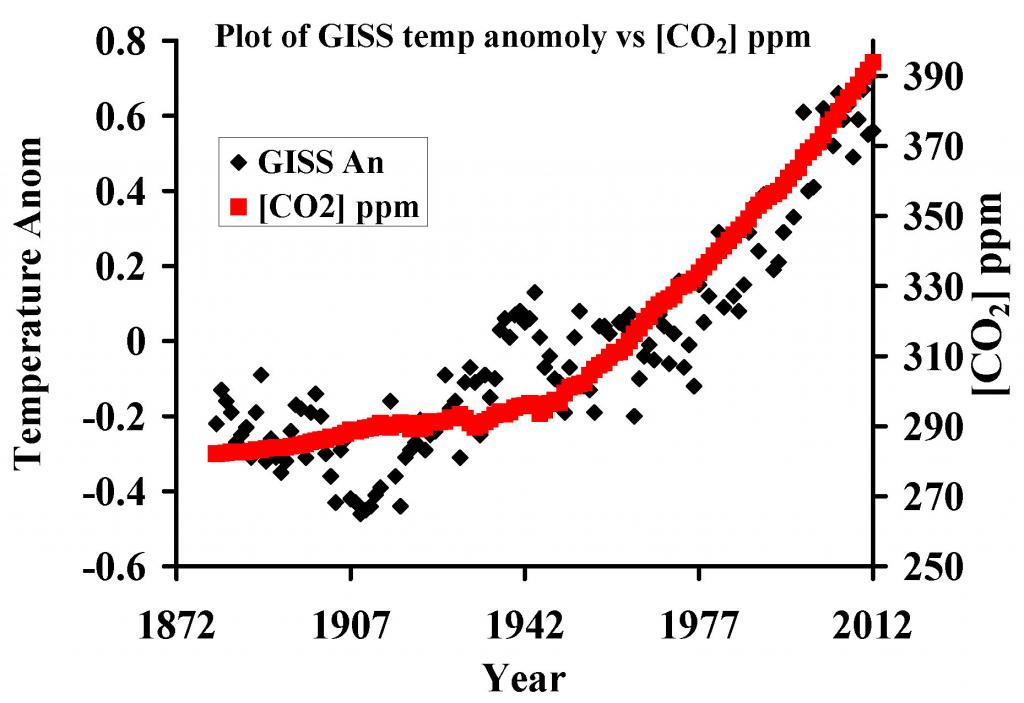
To overcome the poverty of hindcasting and to aid forecasting, I decided to improve the length of the study period. Firstly I attempted to come up with an estimate of past atmospheric [CO2] levels, by examining the relationship between the estimates of anthropogenic carbon released into the atmosphere (Marland & Andres) and the Keeling curve (Keeling & Tans), Figure 1.

Figure 1 shows the 1969-2012 Keeling CO2 curve and the historic and modern estimates of anthropogenic carbon produced by Marland&Andres. The red points are the actual levels of CO2 measured by Keeling and co-workers and the blue represents my estimate based in the estimates of total man-made CO2 sources.
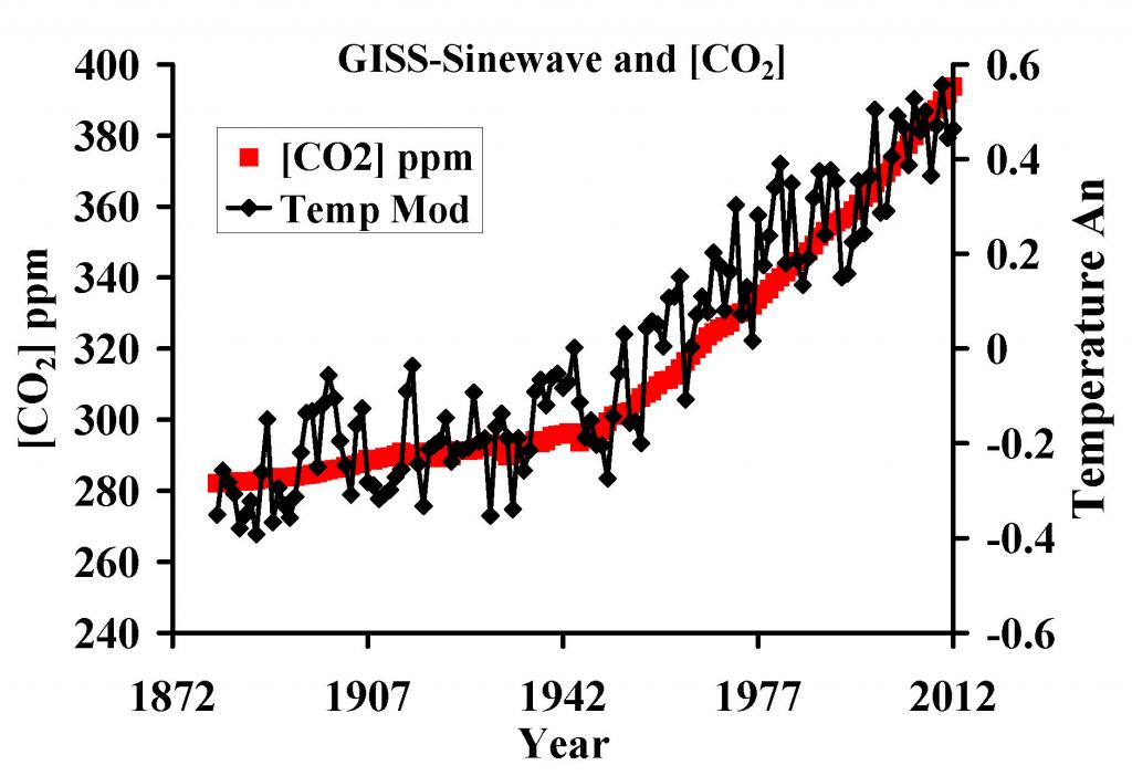
The estimated and measured atmospheric CO2 and GISS temperature from 1880 and 2012 is shown in Figure 2.
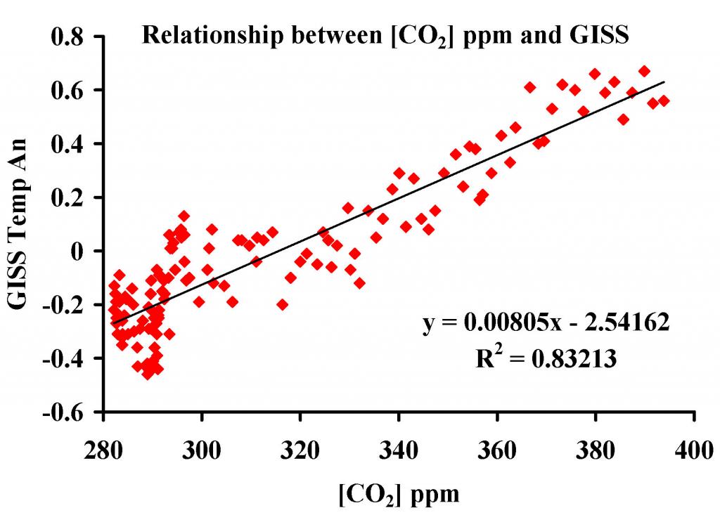
Then [CO2] is plotted against the GISS global temperature anomaly, which is shown Figure 3.
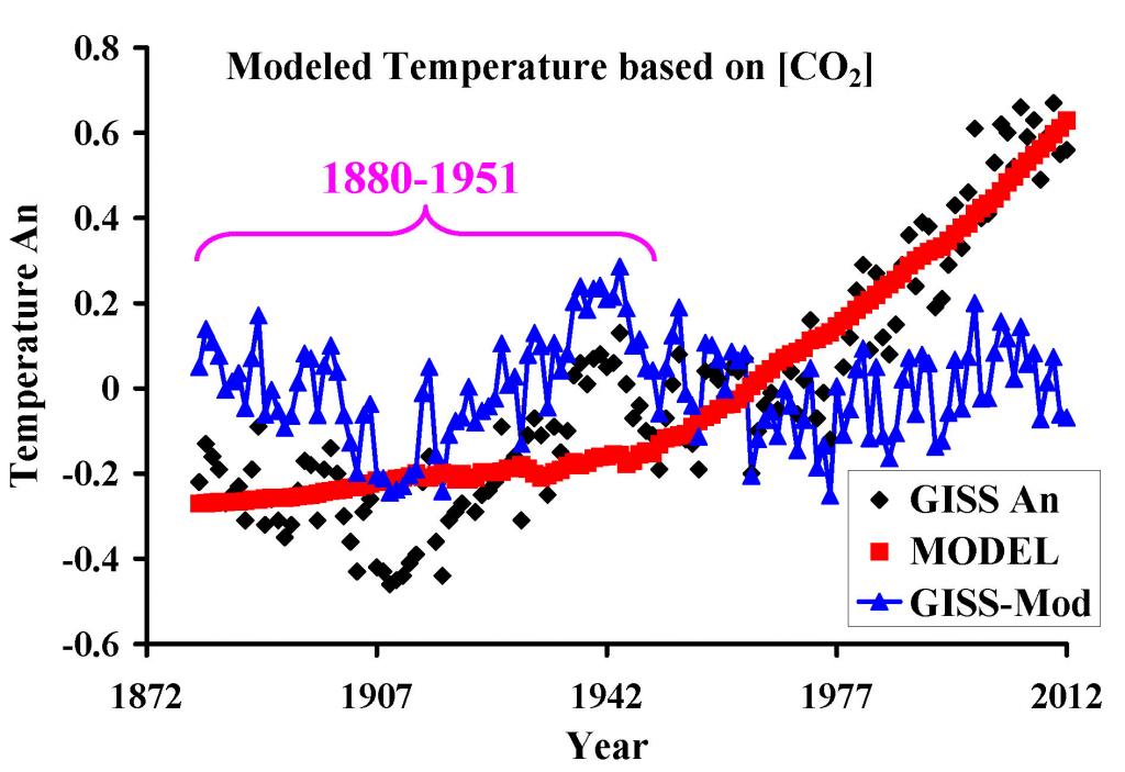
From Figure 3, the red line represents what the temperature would have been if 100% of the temperature change was due to CO2. The black points are the temperature anomaly estimates of GISS. Thus, we can plot the residuals, in blue, from the curve, real minus model, shown in Figure 4.
The nature of the residuals in the years 1880-1951 appears to be cyclic, and is shown fitted to a sine wave, with peaks/troughs 63 years apart (+/- 0.14 degrees), Figure 5.
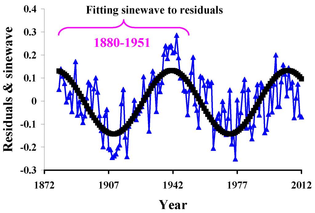
What is nice is that the sine-wave generated based on the 1880-1951 fits the 1951-2012 very nicely. We can take out the sine-wave from the GISS data and see how the Earths temperature would have been if this, possibly mythical, cyclic hording and then thermalization of heat is removed. When plotted with CO2 the line shapes are rather close, Figure 6
With this, possibly mythical, cycle removed we can now plot the logarithm of estimated CO2 vs. estimated temperature, and directly calculate climate sensitivity, Figure 7.
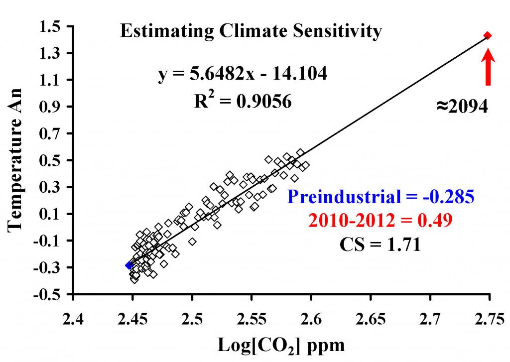
The climate sensitivity comes in at about 1.7 degrees, with 0.78 of this rise already observed. This will happen in about 2094. However, the temperature in 2094 need not represent the pre-industrial temperature plus 1.7 degrees, because of the heat oscillator. We can both hindcast and forecast based on the climate sensitivity and the sine-wave we identified, Figure 8.
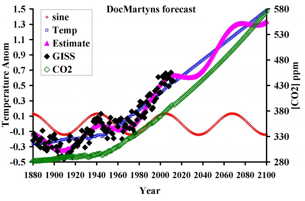
In Figure 8 the green line is the estimate of atmospheric CO2. The blue line is the estimate of the rise in temperature caused by CO2, using a climate sensitivity of 1.7. The red line is the cyclical component. The purple line is my hindcast and forecast of temperature, based only on a cyclic component and atmospheric CO2. The black diamonds are the GISS data points and these match the model almost perfectly.
My forecast, based on graphology and making no attempt to base the cyclic component on any know physical process, is that temperatures will remain flat until 2040.
JC note: This is an unsolicited post that I received via email. This is a guest post that reflects only the opinions of DocMartyn. Please keep your comments relevant and civil.

Now, if we can get beyond the old, ‘if you don’t work you don eat’ business…
no one needs to bother with making up scare stories about global warming and dying polar bears.
Thanks DocM, and Doc C, for putting this up. It would be nice to know Judith, what you think of the work. You’re objective and as I’m lacking the ability to make a determination of my own, someone I trust. We non-scientists have to make decisions as to who we trust, something I think is perfectly legit.
Care to comment?
DocMartyn’s estimate of climate sensitivity and forecast of future global temperatures
Posted on May 16, 2013 | 1 Comment
by DocMartyn
“My forecast is that temperatures will remain flat until 2040.”
I will bet dollars against donuts your forecast won’t survive the week. Global average temperature reliably rises as the northern hemisphere spring and summer progresses.
Doc,
1.You say your forecast is that “temperatures will remain flat until 2040.” It looks like your Figure 8 shows temperatures remaining flat only to 2030.
2. You may want to label your charts with figure numbers.
David, don’t you think a week is rather a small time period to invalidate a model?
I understood some 13-17 years was now vogue.
It might be Big Dave’s way to express concerns about the expression ‘temperatures’ in your forecast, Doc.
I had not thought that Temperature Anom., and An., really required explicit definition.
I you specified a smoothing interval I missed it. Is a year too short? I don’t know. It’s your prediction not mine. Seventeen years seems a bit long to dodge accountability.
Why don’t you go ahead and specify exactly what would constitute a failure of the prediction?
That is a very good point David. I was thinking about Lucia’s recent plotting of the AR4 ensemble verses measured temperature change and trying to think of a robust statistic to indicate a fitting failure.
It is quite obvious that one should compare the statistical variation of real-model in the hindcast with the same statistical variation with the revealed forecast. However, the temperature anomaly is measured in different placing, using different instruments and is calculated from different instrument densities, throughout the record.
I would be very happy if you, or anyone one else, were to suggest a metric that one could apply to my own little endeavor and to mainstream models, allowing them to be declared falsified.
If I had a suggestion I would have given it to you already. I’m not exactly shy. Your hypothesis your responsibility to describe how it may be falsified. If it can’t be falsified it has no explanatory power. A theory that explains everything explains nothing. Evolution is worse as the emergence of novel biological structures make glaciers look like they move at warp speed. Welcome to never-ending debate where goalposts are always moved upon approach. Are we having fun yet?
I see a lot of data points and curves but no physics. Everything hinges on secondary effects and feedbacks. Over the pas couple of years we have been presented with numerous analyses, arguments, claims and diatribes. The bottom line is that we remain ignorant.
Yeah that’s my take. The bottom line remains that whatever happens we’ll have to find a way to deal with it because the only sure thing is that a political means of curtailing CO2 emissions enough to matter is not possible. Feel-good measures to reduce it in the US and Europe are just monumental wastes of money, time, and talent. Lomborg gave the only possible answer in recent testimony before congress. Find a cheaper source of energy that doesn’t emit CO2. That has to be done regardless at some point so every bit of effort given to inevitably insufficient mitigation of fossil fuel burning just makes the situation worse. A vibrant growing world economy is what provides the funding for big science. The solution must be technological not sociological. The global village thing where everyone wears Birkenstocks and survives by growing vegatables in their backyard is not happening. The sooner the moonbats get that fantasy out of their heads the faster the rest of us can proceed in finding a solution that actually works.
I mostly agree with this summary of the situation. I’ve tried to come up with more-neutral labels for these two positions and am going with Optimistic Fatalists versus Urgent Mitigationists. OFs believe that it’s all going to get burned until something that is (privately) cheaper and better comes along.
A vivid way of stating this hypothesis is that when the quantity of fossil fuels burned actually does collapse it will be during a period of falling fossil fuel combustion prices, not rising ones. The peakers and UMs generally believe the opposite (although the UMs fantasize that the rising combustion price at the end will equal the fuel price plus a carbon charge, with the sum increasing but the fuel price possibly falling).
1.7C doesn’t sound like much but what happens when we take geographical distribution into account? The tropics aren’t warming. The southern hemisphere is warming much less than the northern. Continents are warming far faster than the ocean. What it looks like is that the 1.7C translates into some very steep temperature rises in the higher latitudes of the northern hemisphere and no notable change elsewhere. What should be studied are the consequences of the lopsided distribution of “global” warming and that’s probably not very practical given the state of the science today. Therefore I continue to support Bjorn Lomborg’s view that all due haste and priority be given to finding a less expensive energy source than fossil fuels. A less expensive source of energy doesn’t have to be forced upon an unwilling short-sighted world. Such a forcing is a political impossibility so Lomborg’s answer is the only possible way out of the pickle we’re getting ourselves into if indeed it is a pickle and not a blessing in disguise. I’m not convinced the warming will be a net negative. People don’t like the winters much where I grew up and the non-human fauna find it a near catastrophic annual struggle to survive the snow and the cold.
“People don’t like the winters much where I grew up and the non-human fauna find it a near catastrophic annual struggle to survive the snow and the cold.”
The arctic peat-lands sequestration of carbon,decreased from the MCA during the LIA.The negative feedback of warmer T on the peat lands and the Siberian bogs is significant on the atmospheric fraction.
Believe me, Mr Springer!
If the brunt of global warming happens in the mid-latitude northern hemisphere we can deal with it easily. In fact we will relish it.
We are even inventive and resourceful enough to make it an asset, not a catastrophe.
Also – we could certainly use some fair weather.
A fitting exercise using past 140 years for forcasting the future 90 years….
the time frame is much too short. Plus,The Scafetta-cycle is 61 years,
shorter than 70 years reckoned…..
Possibly, how ever I put this together before I read the words of Kevin ‘missing heat’ Trenberth:-
“One of the things emerging from several lines is that the IPCC has not paid enough attention to natural variability, on several time scales, especially El Niños and La Niñas, the Pacific Ocean phenomena that are not yet captured by climate models, and the longer term Pacific Decadal Oscillation (PDO) and Atlantic Multidecadal Oscillation (AMO) which have cycle lengths of about 60 years.
From about 1975, when global warming resumed sharply, until the 1997-98 El Niño, the PDO was in its positive, warm phase, and heat did not penetrate as deeply into the ocean. The PDO has since changed to itsnegative, cooler phase.
It was a time when natural variability and global warming were going in the same direction, so it was much easier to find global warming.
Now the PDO has gone in the other direction, so some counter-effects are masking some of the global warming manifestations right at the surface.
http://davidappell.blogspot.com/2013/05/my-article-on-temperature-hiatus.html
The AMO appears to have quite an nice 60ish year cycle, following my Fig 5.
http://www.nature.com/ncomms/journal/v2/n2/full/ncomms1186.html
Figure five of this paper has this rather interesting graphic,
http://www.nature.com/ncomms/journal/v2/n2/fig_tab/ncomms1186_F5.html
which shows a periodic deconvolution of a number of temperature related proxies, in different locations, with periodicities centered around 65 years.
Chambers et al, 2012 have a nice graphic looking at a 60-year oscillation in global mean sea level, with a very similar sinewave, and centered in the same phase as one I fitted.
http://onlinelibrary.wiley.com/doi/10.1029/2012GL052885/abstract
The figure from Chambers et al., is here:-
http://cyclesresearchinstitute.files.wordpress.com/2012/11/60-year-sea-level-cycle.jpg
I will point out that this is a fitted hindcast based on fixed cycle of fixed amplitude and fixed length, with a linear relationship between Log[CO2] and Temperature.
Based on fit, I made a predictive model. I had a look at what may generate a 60 year warming/cooling cycle later.
“Atlantic Multidecadal Oscillation (AMO) which have cycle lengths of about 60 years.”
Kevin ‘missing heat’ Trenberth is suggesting that ghosts are the cause of variability,Spooky.
http://www.nonlin-processes-geophys.net/18/469/2011/npg-18-469-2011.html
To put it another way, as chance is also a cause of cyclic processes eg Slutsky.
http://carlo-hamalainen.net/stuff/Slutzky%20-%20The%20Summation%20of%20Random%20Causes%20as%20the%20Source%20of%20Cyclic%20Processes%20%281937%29.pdf
Obviously we need a better understanding of random dynamical systems.
there is a nice paper on the ramifications of policy and forecast error from broadbent at the BOE.This is a remarkable document of equal standing to Haldanes dog and the Frisbee paper,
http://www.bankofengland.co.uk/publications/Documents/speeches/2013/speech653.pdf
Maks, Phantoms of the Greenhouse. I like it.
As a policy economist, I’ve often said that we can’t sensibly make long-term economic forecasts or projections, and that it is not sensible to base policy on them. The speech by Bank of England economist Ben Broadbent, a former Treasury forecaster, strongly supports this stance. Broadbent notes that “even when we look only a year ahead, the unpredicted component in annual GDP growth – the “noise” – has been significantly greater than “signal” we’re able to extract from the various economic indicators, and on average close to twice as big. … the economy has always been volatile. … we also have to accept that, to a significant extent, many objects of interest, including GDP growth, are genuinely unpredictable, comprising at least as much noise as signal.”
When it comes to forecasting the occurrence of infrequent events, Broadbent notes that “Whether it’s the simple frequency with which they occur, or a more sophisticated understanding of the risks of their occurrence, we need quite a bit of data to uncover these things with any degree of precision. In the meantime, it probably won’t be possible to make decisive comparisons between forecasters: you’re likely to have to go through several events, and wait a long time, before deciding which is better.”
Broadbent says that “We are … as the psychologist Daniel Kahneman puts it, “machines for rushing to judgement”, biased judgement at that. We are naturally too inclined to see structure in what is actually random.” This applies, of course, to all facets of life, including global temperature analysis. In his conclusion, Broadbent states that: “At the same time, we should remember that it is only through forecast errors – by coming across things we hadn’t previously thought of – that we discover more about the world. “We should be pleased with forecast failures,” says Sir David Hendry, the distinguished econometrician, “as we learn greatly from them”. Yet, in reality, we do not always find it a pleasing experience. We all of us prefer to be right and are made uncomfortable by events that don’t fit into a coherent model of the world, preferably the one we already hold in our heads. Psychologists tell us that these instincts are so deep-seated that they often over-ride our rationality: we wishfully see structure in random events; believing this structure, we are often over-confident about our own predictions; when it comes to others’, we are too quick to assign significance to their forecasting errors, whether small or large. If the forecast turns out to have been correct we immediately assume the forecaster is good; when it’s wrong we are quick to blame the forecaster rather than chance. As we saw with some of the simulations [in the speech] it can, with enough chance, take a very long time to tell apart a “good” from a “bad” forecast, but our instincts often jump the gun.”
Judith, perhaps Broadbent’s paper would make a good head-post?
Banks?
How about telling the insurance companies to fire their actuaries :
http://www.nytimes.com/2013/05/15/business/insurers-stray-from-the-conservative-line-on-climate-change.html
I suppose they just guess, right? Or do the actuaries read this blog’s comments section and plan according to whatever The Chief says?
Or perhaps the actuaries do things like modeling, simulation, and statistical analysis. and try to do it better than their competitors?
I don’t know, just asking.
WHT, your linked article says that “the focus of insurers’ advocacy efforts is zoning rules and disaster mitigation.” That is, limiting exposure to untoward events and increasing capacity to deal with then should they arise. Not unrelated to my arguments for policies which don’t depend on a specific scenario for the future but which increase our capacity to deal well with whatever eventuates. Policies which support flexibility of response.
The article also says that “Mr. Muir-Wood notes that the insurance industry faces a different sort of risk: political action. “That is the biggest threat,” he said.” Which could be taken to support my preference for smaller government and more self-reliant individuals and non-government bodies; again, actions which promote resilience whatever befalls and which are less dependent on political whims.
Faustino said in his post on May 16, 2013 at 10:28 pm
“As a policy economist, I’ve often said that we can’t sensibly make long-term economic forecasts or projections, and that it is not sensible to base policy on them. The speech by Bank of England economist Ben Broadbent, a former Treasury forecaster, strongly supports this stance.”
__________
Then you must believe it’s not sensible to have long-term policies since policies are based on some expectation about the future.
I’m not sure Broadbent’s speech supports your stance. I’ll quote some of his closing remarks.
“I should certainly not leave you with the impression that economic forecasting is so inaccurate that we shouldn’t bother with it. For one thing, we have to: central banks cannot avoid making judgements about future risks, in some form or other, because monetary policy only works with a lag. As Alan Greenspan put it some years ago, “Implicit in any monetary policy action or inaction is an
expectation of how the future will unfold, that is, a forecast” (see also Budd (1998)). Second, the usefulness
of the Inflation Report process extends well beyond the production of the fancharts: it facilitates a detailed
discussion of the implications of alternative policies and allows the MPC to communicate its views to the
public.”
http://www.bankofengland.co.uk/publications/Documents/speeches/2013/speech653.pdfhttp://www.bankofengland.co.uk/publications/Documents/speeches/2013/speech653.pdf
Max, we’ll usually have some sort of view of the future. The IPCC’s various scenarios were based on (discredited) economic modelling of the economic growth of each country from 1990-2100. Estimates of net costs by Stern et al are based on outcomes in 100-150 years. I have argued that at no time in history would a forecast for 90-100 years ahead have been remotely accurate. More recently, forecasts in 2000 of the economic situation in the major economies – the US, the EU, China and Japan – in 2013 would have been hopelessly wrong, those for, say, Egypt and Syria would have been worse. Broadbent is concerned mainly with short-term forecasting, and he points out the difficulties in assessing the merits of alternative long-term forecasts before many years have passed – if we can’t determine until, say, 2080, that forecasting technique or model A is superior to technique or model B, the we have little basis for choosing one in 2013.
In economic modelling to compare, for example, the impacts of different policies or of a government-subsidised major project, a ten-year horizon is generally used. This doesn’t produce projections for a decade hence, it says that, within certain confidence limits, we would expect a certain difference in outcomes between different policies or from project X over ten years. I have argued that the future is always highly uncertain and that our capacity to forecast even 20 years ahead is very limited, and that it makes no sense to adopt costly policies on the basis of what might be 80-100 years ahead. Instead, it makes sense to adopt policies which allow us to respond to whatever befalls, e.g. with flexibility from open markets, limited regulation and policies which foster innovation, entrepreneurship and self-reliance. Such policies will serve us well whatever the future holds.
I have been an economic policy adviser to the UK, Australian and Queensland governments, with a focus on drivers of economic growth, and I have seen time and again the dangers in high-spending, long-term government projects, e.g. Australia’s current NBN (broadband network), which largely ignores the advance of wireless technology and is spending perhaps $A40-50 billion to very slowly roll-out what is likely to be outmoded technology at high cost to the community and any eventual users. The IPCC process is an invitation to governments to adopt costly long-term projects which they are ill-equipped to design or manage. A system which allows decentralised decision-making by those with skin in the game and relevant knowledge and expertise is likely to produce far better results, and will be more adaptable when forecasts inevitably prove wrong.
By far the most successful governments in promoting growth in the economy, employment and opportunity in Australia have been the Hawke and Howard governments which largely adopted the approach I favour. Conversely, the most centralising governments, with opposite beliefs, have been the most disastrous – Whitlam, Rudd, Gillard. The EU is a classic case of centrally-driven sclerosis where bureaucracy prevails over flexible, entrepreneurial approaches. It’s no surprise that the forecasts made by these latter examples are wildly wrong.
Faustino said on May 17, 2013 at 11:45 am
“Max, we’ll usually have some sort of view of the future.”
___
Well, Faustino, your view of the future would be a forecast, but you said earlier
“As a policy economist, I’ve often said that we can’t sensibly make long-term economic forecasts or projections, and that it is not sensible to base policy on them.”
I am puzzled by your statements. Perhaps you are saying you don’t believe long-term economic policy is sensible because long-term forecasts are not sensible, even your own?
You also said: “I have argued that at no time in history would a forecast for 90-100 years ahead have been remotely accurate.”
Have you evaluated the accuracy of all 90-100 year forecasts made 90-100 years ago and even earlier?
That
WHT,
Insurance and their web of paper packagers make huge money off of fear, in fact all of their money.
Immediately after Katrina they met in the Bahamas and then and there they decided to raise the fund for hurricane damage 60 billion dollars, based on what the alarmist told them. They have no plans to return the money.
True, true Nicola Scafetta demonstrated the accuracy of fitting to historical temperature records a 60-year sinusoidal curve with a 0.25°C amplitude, peak-to-trough, that corresponds perfectly with the periods between the 1880-1940 and 1940-2000.
[“Empirical evidence for a celestial origin of the climate oscillations and its implications,” Journal of Atmospheric and Solar-Terrestrial Physics (2010) ]
It’s a poor man indeed not worth his own climate sensitivity.
===============
If this forecast is correct, it means I am going to have to listen to people’s b.s. scare stories again from 2045 to 2065.
There are many things left unexplained here.
1. Why does your Figure 1 show the CO2 curve only from 1969 on. The Keeling measurements started in 1958.
2. Where are the links to the various papers (Marland and Andres,Keeling and Tan, etc.?
3. Where are your data? Excel files, please.
Judith, both Science and Nature have now adopted a policy of requiring authors to provide their data on submission of the papers. (Also the code, although they seem to be wishy-washy about enforcing that.) Don’t you think that your blog is at least as worthy and morally correct as those two magazines? Why not institute a policy like that for persons submitting guest blogs?
Good to see alternative approaches taken.
DocMartyn is looking at ocean plus land.
The fifth figure shows a linear regression yet he later computes the logarithmic sensitivity. Why not do a log regression in the first place? I ask this because based on the theory, the temperature should bend logarithmically with increasing CO2. He does this later but only after removing parts of the temperature signal. Really should keep this consistent, so we can see whether that had an effect.
Overall it is pointing to a 2.5 C temperature change with a doubling of CO2 when the heat sinking of the ocean is compensated for.
Duplicate the analysis for land-only and you will see the fastfeedback view.
Very similar to to the analysis by BEST and Tamino and others, myself included, so good job.
“Overall it is pointing to a 2.5 C temperature change with a doubling of CO2 when the heat sinking of the ocean is compensated for.”
No Web, no. The fit is over 120 years and the forecast is for the next 90. Please note there is not ‘lag’ explicitly used nor proposed.
I know you are a fan of heat being stored in the oceans and then jumping into the atmosphere following some unspecified time, like a Jack-in-the-Box, I do not agree with your analysis.
i have asked you before where this 0.8 degrees is going to hide and when it is going to emerge thermalized.
With a rhythmic, oscillation of heat storage/heat thermalization, one has already covered this base.
It is a thermal forcing and will only gradually emerge as an elevated temperature. Hansen has acknowledged this fact way back in 1981and perhaps earlier. The model is describing equilibrium climate sensitivity and that is the way the physics of the environment is playing out.
Web. have a look at this
http://ars.els-cdn.com/content/image/1-s2.0-S0277379108003740-gr2.jpg
Depth profiles of seasonal temperature, salinity and dissolved oxygen concentration at 22.5°S and 161.5°E under modern climate (Levitus and Boyer, 1994)
Would you tell me how heat is going to ‘equilibrate’ under the thermocline and change the seasonal line shapes ?
Just model it there a good chap.
Doc Martyn ‘s chart throws some light on the
dark ocean depths and the travesty of that
pesky missing heat. Tsk, perhaps yer should
get inter yer bathyscaphe and take a look,
WebHubTelescope. Btcg
This is the climate sensitivity for the land, while attempting to approximate DocMartyn”s approach, but using only the BEST data.
http://img197.imageshack.us/img197/2515/co2sens.gif
Note that it comes out to 3.16 C for doubling of atmospheric CO2 levels. That is right in line with the mean estimate from all models, all the way back to Hansen’s prediction in 1981.
The combined ocean+land will be about 2/3 of this value, as the ocean sinks a portion of the excess heat.
That’s what the models say, can’t deny that fact.
Heat stored in the oceans is stored there, in the relevant time scales of these discussions, for good. Most of it.
It’s not jumping back out to get us.
Change in OHC is hypothetical. The instrumentation we have is incapable of unambiguously resolving such relatively tiny change in OHC. It’s too dilute and coverage is insufficient both spatially and temporally. This was demonstrated when ARGO data was massaged a few years ago and the massage changed its polarity. If it can be pencil whipped from one polarity to another it’s too small to reliably measure.
The passage of heat through the upper to the lower somehow escaping detection on its way down borders on farcical and, as you point out, this stored energy somehow reemerging to warm the atmosphere is a ridiculous proposition. Climate science is a big joke. No one with any sense takes it seriously. It’s a means for leveraging other agendas like keeping funding flowing into the academy, raising taxes, generating and exploiting subsidies for alternative energy schemes that won’t work, and so on and so forth.
Web, think on this. The whole globe has 70.5% water and 29.5 land. The NH has 60% water and 40% land, the SH has 91% water and 19% land.
The slope of a plot of SH vs NH temperature anomalies gives a slope of 0.81.
A back of an envelope calculation suggests that the CS of the oceans is 1.28 degrees per doubling and for land is 2.7 degrees per doubling.
If we perform the same analysis as above, using the BEST land only data, I believe that should, a prior, find the same sinewave and also a climate sensitivity of 2x[CO2] of about 2.7 degrees.
I will have ago later in the evening and see what the CS of the BEST dataset is. I predict it will be about 2.7.
As David Springer demands a exact falsification, a prior, criteria, I will go for 2.7 +/- 10%, or 2.7 +/-0.27 degrees for the 2x[CO2] on land, where it is not noisy, from 1850 onward.
Regardless of current or previous theories, the Arctic sea ice declined dramatically after the Napoleonic Wars. Nobody knows why, and because it’s not a favourite subject, nobody is trying to find out why.
Later in that century, after sea levels had risen sharply, in a process which started before the Napoleonic Wars, Arctic sea ice nonetheless increased dramatically. Nobody knows why, and because it’s not a favourite subject, nobody is trying to find out why.
Arctic melt after WW1? Hotter world for a bit? Arctic temps plunge in the sixties, big advance of ice in the seventies? Arctic goes all melty again after the abnormal “norm” of the 70s, yet not nearly so much SLR as a couple of centuries ago? Nobody knows why, and because it’s not a favourite subject, nobody is trying to find out why.
Now we have handy but hopelessly rough observation sets like ENSO, PDO etc treated as climate “mechanisms”, locked in some sort of arm wrestle with GHGs. Maybe if we banned acronyms for a bit…
How is it we are so ignorant and uncertain about past events yet so knowledgeable about what is going to happen? Is it because the future does not have a voice to contradict our theories, unlike that pesky past?
Stop predicting. Just stop. Straight out. Don’t predict. What you don’t know, you don’t know. As for gang-review and Publish-or-Perish, why not get in early and disbelieve today? You’re going to do that anyway, right? Before the warranty is up on your cheap Hyundai, that solemnly announced “paper” or “article” is one with Nineveh and Tyre.
So disbelieve now and beat the rush.
mosomoso,
Can’t give yer a ‘plus one,’ fer reasons I prefer not ter go
into. Contrary ter what Yogi Berra says about the fucher.
seems it’s more difficult ter predict the past than predict
the fucher.
‘So disbelieve now and beat the rush.’ Lol, I do and I did!
A serf
Well given that i have spent a good long while criticizing other people models it was only fair to give others a chance.
I just wanted the simplest model that would capture the effect of atmospheric CO2 as a ‘GHG’ and also capture the nature of ocean oscillating warm/cool cycles, which the GCM’s seem to have missed.
The fact is that temperatures are flat over the last decade, CO2 has risen, and the GCM’s have missed this ‘pause’. A natural downward dip in temperature is being balanced by the re-radiated IR flux from increasing CO2.
I have just assumed that the past is a reasonable guide to the future.
I think it would be nice if people who claim higher climate sensitivities and very large lags between changes in energy fluxes and temperature, would present their hindcasts and forecasts in a similar manner to my final figure.
How does your model compare with Dr. Akasofu’s graph?
http://wattsupwiththat.com/2009/03/20/dr-syun-akasofu-on-ipccs-forecast-accuracy/
DocMartyn | May 16, 2013 at 8:46 pm | Reply Well given that i have spent a good long while criticizing other people models it was only fair to give others a chance.
I just wanted the simplest model that would capture the effect of atmospheric CO2 as a ‘GHG’ and also capture the nature of ocean oscillating warm/cool cycles, which the GCM’s seem to have missed.
As I do not see how Mauna Loa can be measuring anything but local production and the history of agendas show their CO2 rise was from a cherry picked low start date and the manipulation of data from that obviously continue, in other words, there is nothing to show there has been any rise at all in global CO2 levels as based on this mythical, unproven, “well-mixed background” concept – is there any way you, or anyone else, could put together a graph showing how the temps relate to all the known cycles which the models fail to include?
I see this in dribs and drabs, but visualising the combination of them beyond my ken of them.
Myrrh, Keeling and his group stand out as outstanding scientists who work on very difficult problems. I have looked through many of his publications and publications of his colleagues and one can see they are very cautious in their claims for instrument design and measurement.
Their sampling and calibration routines, including testing their own standards and publishing errors identified due to their standard gas mixtures being below specification, indicate that they are dedicated, hardworking and honest scientists and people.
mosomoso, well said, your fifth para is addressed to an extent in some of the quotes I included in my above post.
mosomoso, scientists may understand more about the history of Arctic sea ice than you think. Below is a link to a Quaternary Science Reviews article titled History of sea ice in the Arctic, which you may enjoy reading. The following quote is from the article:
“Reviewed geological data indicate that the history of Arctic seaice is closely linked with climate changes driven primarily by greenhouse and orbital forcings and associated feedbacks. This link is reflected in the persistence of the Arctic amplification, where fast feedbacks are largely controlled by sea-ice conditions(Miller et al., 2010). Based on proxy records, sea ice in the Arctic Ocean appeared as early as 47 Ma, after the onset of a long-term climatic cooling that followed the Paleocene–Eocene Thermal
Maximum and led to formation of large ice sheets in polar areas.”
____
mosomos you say: “Stop predicting. Just stop. Straight out. Don’t predict. What you don’t know, you don’t know.”
You are predicting it would be better if we stop predicting.
I like your sense of humor.
http://bprc.osu.edu/geo/publications/polyak_etal_seaice_QSR_10.pdf
Oh, Max, I don’t want to get all technical here, but I am not predicting it would be better if we stop predicting. I am commanding. Furthermore, nobody is to try wriggling around my command by just projecting. Predict…project…it all has to stop. The Nile priests excelled all others in this type of thing – and they still sucked. So I’m banning!
Also, any publication caught using the words “greenhouse”, “forcings” or “feedbacks” is banned for extreme juvenility and mindlessness. The above words are not as bad as “ideation” – but no word is, not even “normative”. Banned!
Because I am above my own laws I will make the odd prediction. For example, I here predict that the climate in 2040 will be profoundly different to that of 2030 or 2050. That’s actually dead easy, since climate is nothing but change, and over any decade it will do cartwheels, as it’s always done.
You may go now.
mosomoso, I can easily beat you forecast.
I forecast average global temperature in 2040 will be higher or lower than it was in 2030, if not the same. Furthermore, I forecast the average in 2050 will be higher or lower than it was in 2040, if not the same. Finally, I project the average in 2050 will be higher or lower than it was in 2030, if not the same. I guarantee my forecast will be accurate.
Try topping that !
Try
This year’s Melbourne cup will be won by an odd-toed ungulate mammal with more than three and less than five legs. (Me et al. 2013)
Horse racing is tricky, because, instead of politely pretending you never spoke or published, they actually check the result. Ehrlich and Gore have it easy.
Source: me (Does that sound all sciency, or what!)
DocMartyn says: ”My forecast is that temperatures will remain flat until 2040”
is that for how long you intend to leave Doc? Co2 is produced beyond anybodies expectation – if is not increasing the temp now, never will.
You have learned from Nostradamus, same as the rest of the swindlers: predict something for after you are gone – cheap trick. .Why bothered, to only expose your shallow knowledge…?
Well I nailed my colors to the mast. Should we see an increase of >0.2 degrees per decade, over the next 20 years or so, I will wear sack-cloth and ashes and become an evangelical ‘Thermogeddonist’.
+1
A priori, the calculation of climate sensitivity should be trivial. The ability of CO2 to absorb infra-red radiation is a function of the logarithm of its concentration and therefore one could make a plot of Log[CO2] vs. temperature and from the slope estimate the climate sensitivity directly.
This ignores the fact that the lower atmosphere is already opaque to infra-red in the CO2 absorption bands. Heat is transported upward through the atmosphere by convection not by radiation as confimed by the observed adiabatic lapse rate. This heat is then radiated into space above the tropopause at around -18 deg C as predicted by Stephan’s Law. How would increased CO2 affect this process?
Lapse rate is largely fixed as a macroscopic property of the atmosphere and the planets gravity, so that the entire temperature profile is shifted upwards but remains co-linear. With more CO2, the infrared escapes at higher altitudes where it is colder, the earth has to heat up to provide enough outgoing thermal radiation to reach steady state.
This is a recent derivation of the lapse rate for both Venus and Earth that is suitable for a college course in atmospheric physics:
http://theoilconundrum.blogspot.com/2013/05/the-homework-problem-to-end-all.html
The observed lapse rate is off by 50% from the classical derivation assuming an adiabatic process. This derivation fills in the details.
Poppycock!
Take the poppycock with two cents and a grain of salt.
Certainly the lapse rate differs in highly mountainous regions, as you will find many references to variations in lapse rate in physiology journals. There they justify the research to warn mountain climbers and other high-altitude researchers not to trust the lapse rate numbers.
Elsewhere, it seems as if the lapse rate is standardized. The same numbers were used back in 1930 for designing superchargers for aircraft:
[1]O. W. Schey, “The comparative performance of superchargers,” Report-National Advisory Committee for Aeronautics, no. 365–400, p. 425, 1931.
The same standard is used today even though CO2 levels have gone up by 40%.
I think AK and I are talking about different things. I am talking about an average lapse rate, while he is talking about extreme conditions.
I am still looking at verifying my derivation for establishing the standard lapse rate for the lower atmosphere, which seems to work well for climates with a net greenhouse atmosphere, so it works for Earth, Venus, Mars, and Titan.
http://theoilconundrum.blogspot.com/2013/05/the-homework-problem-to-end-all.html
It doesn’t work so well for the outer planets with a net radiating-out atmosphere. That includes Neptune, Uranus, Jupiter, and Saturn, where the standard adiabatic derivation works fine from what I can tell. Those atmospheres are completely transparent to the net out-going radiation and pick up no thermal energy that way.
I doubt it. In any event, I’m talking about the average lapse rate for the planet, which depends on the detailed evolution of the weather. I’m saying that it probably was/would be different without the local effects of the Himalayas and Tibetan Plateau, as was the case before the Indian Plate collided with Asia.
I’m saying that probably localized geological features have a strong effect on the climate, which can be observed as differences in the average temperature, average lapse rate, average tropopause height, and average thickness of the tropopause (as well as other details).
Given that the lapse rate varies tremendously with latitude (i.e. poleward/equatorward of the Polar Front), whatever “standard” lapse rate was used in aircraft design included a large range of variation. Changes to the distribution of that variation in space and time could produce large changes to the average lapse rate.
I’ve mentioned this before. Your
hypothesisspeculation requires much more than brushing off contrary data the way Mann did/does.That is worth pursuing. I would agree that definitely the height of the tropopause depends with latitude. In fact, the tropopause height is proportional to the mean tropospheric temperature; that is a rule of thumb used by pilots and meteorologists.
One way for this relationship to hold is for the lapse rate to be constant across latitudes.
Sure enough, this is what research has found out:
[1]P. H. Stone and J. H. Carlson, “Atmospheric lapse rate regimes and their parameterization,” J. Atmos. Sci, vol. 36, no. 3, pp. 415–423, 1979.
However, that paper does reveal that there are deviations with latitude and with pressure as the altitude changes, which is indicative of instability of atmospheric layers. I will keep researching along these lines. As a loyal marxbot, thanks for the tip.
Perhaps, if you’re talking about tropospheric lapse rate. However, the height of the tropopause varies tremendously, especially relative to the characteristic height(s) of radiative surfaces. When you start talking about radiative surfaces, you need to factor in the essentially zero lapse rate of the lower stratosphere poleward of the Polar Jet Stream. This will lower the average lapse rate (at that point) considerably.
I am not referring to the stratosphere. I am talking about the linear decrease of temperature with increasing altitude in the troposphere. That is the constant lapse rate (or gradient) that should be derivable.
On top of that, there is the Poisson’s equation relating pressure, density, and temperature together. The adiabatic exponent of this relation is also off by 50%, which is why it is more often called a polytropic exponent. There is also the barometric formula, which also is dependent on the lapse rate. Lots of altimeters are based on a calibration due to the 6.5 C/km mean.
Where is the derivation for this that shows how it deviates 50% from the adiabatic prediction?
I am just curious.
@WHUT…
In which case it’s highly deceptive to bring it up in discussions of GHG-induced climate change, because that’s irrelevant to issues of the radiative surface.
What are you talking about? The adiabatic lapse rate at 30°C is about 10°/Km. (9.8 per wiki.) It changes a little with temp and pressure, see here. 50% is a very rough estimate.
I don’t know of any reason to expect the actual tropospheric lapse rate to remain constant with changing geography, even if GHG effect remains constant. I see no reason for expecting to find a derivation.
Very interesting that you are not aware that the standard lapse rate is 6.5 C/km and not the 9.8 C/km that students learn how to derive.
There does seem to be a lot of missing energy here. Climate change is partially about energy imbalances (even mostly) so I got curious as to where it went. And I am skeptical of arguments that say 50% is “close enough”.
So my own derivation perhaps has isolated the missing energy as kinetic energy involved in the gravitational attraction, or what is often referred to as virial forces. I was able to derive that 1/3 of the gravitational potential energy goes in this kinetic energy and this can explain the 50% discrepancy. This works for Earth and Venus.
This explanation could be buried in some old paper, but heck if I can find it.
AK, are you an earth scientist by any chance?
Webster, “This explanation could be buried in some old paper, but heck if I can find it.”
I haven’t seen it either and I am not sure virial forces is correct or not, but if you determine the lapse rate for an adiabatic column of air the outward pressure at the base of the column would be greater than the top of the column, since it is adiabatic, that energy is contained to simplify the calculations. In an open system, that outward energy has to be considered. That is the requirement for “isothermal” radiant layers in the up/down radiant models. If that horizontal energy can spread, i.e. not be truly adiabatic, then you have to adjust your model.
Chief uses Ein=Eout +deltaW, where the deltaW is that spread energy required to maintain a constant Eout. You could call it advection, work, whatever depending on your reference. With a spherical shape, the required ratio of W to Eout would be close to constant.
The bad part for being able to use it as a constant is you have to find a layer with stable or near isothermal conditions. This is a point quite a few people have been trying to make, internal energy transfer impacts the radiant models that assume advective transfer it is negligible.
@WHUT…
I’m perfectly aware. The “standard lapse rate” is an observed phenomenon, or rather a standardized value close to the average, which cannot actually be computed because observational evidence is lacking. Sort of like “global average temperature”. The 9.8 value is the adiabatic lapse rate (at ~30°C). The pseudo-adiabat ranges from around 2.5°C/Km (at 40°C at the surface) up to something like 8-9°C/Km at temperatures well below the triple point. In a meteorological system the average lapse rate at any location (within maybe 10-100 Km laterally) will fall somewhere between. The global average is the result of a variety of meteorological processes.
No, I do IT. I have studied meteorology on my own, which is why I find your ignorance or meteorological principles so laughable. It’s sort of like trying to apply the laws of viscous fluids to turbulence. Sometimes, perhaps often, you can model something called turbulent viscosity, but there are very narrow limits to how well this analogy works.
Dry adiabatic lapse rate is fixed on earth at ~10c/km. Mean lapse rate in the tropics is ~6.5c/km and falls under 4c/km with decreasing temperature as you move toward the poles. Arctic is about 4.5c/km and Antarctic interior 3.5c/km.
Following has nice global map of mean lapse rate.
http://ifaran.ru/old/ltk/Persona/Mokhov_pub/LapseRate-FAO06-IACP430.pdf
fyi Geothermal lapse rate away from plate boundaries is 25c/km.
The geothermal rate on earth would be about the same as venus – same rocks, same mass and density, presumably same radioactive isotopes.
The big mistake in saying venus surface temp is due to greenhouse effect is that it’s solar driven – it isn’t – the troposphere on venus is so dense and insulates so well (90 bar CO2 and most of us agree CO2 is much better insulator than nitrogen, right?) that the where the rocks stop the geothermal lapse rate does not and it’s a hotter core by about 1000C (earth estimated at 6000C, venus at 7000C).
I think anyone who tries to make out Venus surface temp as solar-heated is pranking or hasn’t thought it through its geothermal all day long which also handily explains why a planet with a day-length of a couple hundred earth days has an isothermal surface. Day/night equator/pole samo samo temperture on venus and it isn’t horizontal winds as the atmosphere is so thick it moves no faster than ocean currents on earth. Only geothermal heating of the surface can explain it being isothermal so it makes good sense in more ways than one.
Thanks Springer,
The 6.5 value is also referred to as a critical lapse rate. This critical value separates regimes of stability. The fact that it both acts as a mean value across the earth as well as a critical value gives it a deeper significance.
This type of behavior is often associated with an energy minimization, and that’s what I used in my derivation — I minimized the Gibbs free energy function with repect to the thermodynamic variables. That’s how I came up with 6.5 for Earth, 7.7 for Venus, and also a critical lapse rate for the Martian atmosphere.
I haven’t been studying climate science as long as AK or Springer, but this what I got after bearing down on trying to understand the US and InternationalStandard Atmosphere specifications.
“How would increased CO2 affect this process?”
On the face of it, increased CO2 will increase the emissivity of the atmosphere and enhance the radiative atmospheric cooling to space, all the other things being equal.
To John Reid:
Your post seems intellectually honest (unlike many others here) and so I think it merits a response.
Your argument is the oft-cited “CO2 IR absorption is saturated” argument. In fact, as CO2 concentration continues to increase, there are normally very low intensity (low probability) bending mode transitions [ground-state vibration, rotation(n) first-excited-state vibration, (rotation(m)] of higher and lower rotational levels that occur. This means that the absorption band becomes broader. The total energy absorbed by the CO2 is the integral of the absorption band, so a broader band means more of the surface radiation (energy) is absorbed and passed on to the surrounding atmosphere. This slightly increases the temperature of the troposphere, which (by convection and conduction) slightly heats the surface which then emits slightly more IR, including those frequencies that are not blocked by the air, which increases energy loss into space. Thus, the slight increase in surface temperature/IR radiation re-establishes the energy transfer steady state.
If any IR band is saturated, that of the scissor bend of water must be – water is up to 3 or 4% of air in some places. Yet everyone acknowledges the variable greenhouse effect of water as its concentration changes.
The symbol between the two vibrational levels above should be an arrow representing the vibrational transition.
John,
conceptually, the best way to think about why saturation at ground level doesn’t matter is to consider heat balance at the top of the atmosphere (TOA). Here, CO2 is NOT saturated as absolute concentration varies with pressure, and the pressure is low. You can think of this as the altitude where CO2 is no longer saturated and radiation escapes directly to space.
As CO2 increases over time, the effective height at which CO2 is no longer saturated and emission takes place rises, but the temperature of this emission must be the same – the same amount of heat must be emitted.
The lapse rate remains constant, so the temperature of the ground (now further away) must rise, regardless as to whether it is saturated or not at that level.
Bottom line – CO2 does NOT prevent emission from the ground, it raises the altitude at which emission takes place.
That’s all to a first approximation of course. If you want a proper explanation with maths, I suggest the science of doom website which is excellent.
VTallG and WHUT,
Increased altitude for the lapse rate can’t be the full explanation because measured top-of-the-atmosphere, long-wave radiation still shows deep absorptions at water and CO2 frequencies. The main balance must come from enhanced surface radiation at transparent frequencies.
First para above should be in quotes didn’t work
Pretty pictures, but what do they mean? Carbon dioxide seems to be featured but don’t you think it might be over-hyped? Like, giving it credit where credit is not due? I am looking at your charts and you want to take CO2 influence back to the nineteenth century. That will never do because the early twentieth century warming, starting in 1910 and ending in 1940, quite definitely is not greenhouse warming. And this rules it out for all prior occurrences of warming. Just to remind you the rules, laws of physics demand that in order to start a greenhouse warming you must simultaneously increase the amount of carbon dioxide in the air. That is necessary because the absorbance of carbon dioxide in the infrared is a property of the gas and cannot be changed. There was no such increase in 1910. Also, someone must have told you that you can’t stop greenhouse warming suddenly because there is no way to remove all those carbon dioxide molecules mixed with air suddenly. That early warming that started suddenly also stops suddenly in 1940. This means two physical reasons why it cannot be greemhouse warming. But your curves are so sparsely populated with data that this and other important facts cannot be determined by looking at them. I am puzzled, for example, where that sine wave of yours comes from or what it is supposed to tell us. As far as I can see it is just a chance occurrence in a poorly defined part of the temperature curve. I have no idea why you think you can cast the future with such non-sensical graphs. The true story of carbon dioxide is that it cannot warm the world. You may be aware that there has not been any warming for 15 years as even Pachauri himself has admitted. But the amount of carbon dioxide in the air is higher than ever. Greenhouse theory tells that putting carbon dioxide in the air will create greenhouse warming because it will absorb that OLR, that Outgoing Long-wave Radiation, and turn the absorbed energy into heat. We have ideal conditions for that now but carbon dioxide is simply not absorbing it. It is on strike, and Ferenc Miskolczi explains why. He used NOAA weather balloon database to study the absorption of infrared radiation by the atmosphere. He found that the absorption had been constant for 61 years while carbon dioxide went up by 21.6 percent. This substantial addition of CO2 had no effect on the absorption of IR by the atmosphere. And no absorption means no greenhouse effect, case closed. And without the greenhouse effect those pretty pictures of yours mean absolutely nothing.
Great post. Thanks to Docmartin and our hostess.
Quibbles about curve fitting methodology surely abound. So what? A key result is climate equilibrium sensitivity of 1.7, smack dab in the zone of all the many post AR4 estimates that AR5 is likely to ignore. Nice cross validation of yet another interesting perspective.
Now, the Pasteur quadrant question would be, why the derived clomate sine wave? That is the sort of research Dr. Curry was (I suspect) advocating in her last post, and which is sorely needed.
Doc,
It is reasonable to integrate both natural variability and estimates of climate sensitivity to CO2 but how do you know that the estimated thermal response to CO2 was reasonable in the first place ?
If real world sensitivity were to be too small to measure compared to natural variations where does that leave your thesis ?
What would you say if temperatures actually start downward rather than staying roughly flat ?
Faustino’s comment @ 16th May, 10.28pm,
Herewith ‘Faustino the wise.’
While policies leading to only 580 ppm by 2100 would be commendable, I don’t think you should assume they will apply in your warming estimate. Without such policies values in the 700 ppm range should be considered instead and then compared with these lower values to show the effect of these policies, because you effectively assume a per capita drop in global carbon emission to get to your number. I think this will be difficult with population growth and development unless some mitigation takes place leaving fossil fuels in the ground.
In fact, I have a simpler formula that directly relates policy to effect, which is that the warming will be approximately 1 degree for each 100 ppm added. It is a good linear approximation to the most important part of the log curve.
Jim D
IPCC has several “scenarios and storyline”, none of which include Kyoto-type climate initiatives.
The estimated CO2 levels by 2100 run from 580 ppm (B1) to 790 ppmv (A1F1).
In the past, CO2 emissions have more than kept pace with population growth (per capita CO2 generation increased by 20% from 1970 to today).
If we assume that CO2 will continue to rise with population growth and that per capita CO2 generation will increase another 30% from today to 2100, we would arrive at a level of 640 ppmv in 2100. This is would seem like a reasonable “business as usual” projection.
Peter Lang has proposed on other threads that a “no regrets” approach would be to build nuclear plants instead of coal for all future power generation (except in exceptional cases, e.g. for non-proliferation reasons in locations with unstable governments or where the power plant is sitting on top of a coal mine or gas field).
If such a program were really followed, this could reduce the CO2 levels in 2100 by as much as 80 ppmv, to 560 ppmv by 2100.
I believe that there will be a move to more nuclear power (since it is cost competitive today, except in some exceptional locations). Whether the full 80 ppmv are reduced or only a portion, I think it is reasonable to see 640 ppmv as an upper limit, which could be reduced by switching most future power generation capacity from coal to nuclear.
Max
We have to be a little careful, because other GHGs add another 50% to the forcing, but were canceled by aerosol increase in the last century. Aerosol increases can’t be counted on to the same extent with newer energy sources (Hansen’s “Faustian bargain” about the mitigating benefits of sulphates from dirty coal). CO2-equivalent could well exceed 700 ppm when the other GHGs are also unmitigated, and this is the number that matters. The AR5 scenario called RCP8.5 is equivalent to over 1000 ppm CO2e (8.5 W/m2 by 2100), but is not a no-policy path, rather a deliberate path with fossil fuels sustained.
Max_CH, a carbon tax could give nuclear a cost advantage over coal, and give natural gas even more of an advantage than it now enjoys.
I like the idea of paying tax on carbon rather than on my income because I have a small carbon footprint. Also, as you know, I have a financial interest in natural gas.
A revenue-neutral carbon tax is a no-brainer.
Max,
A carbon tax in place of an income tax. There is an idea which I could possibly get behind. In essence it is a form of consumption tax. Theoretically it should encourage savings and investment.
timg56, the linked CBO report discusses ways to keep a carbon tax from being unfair to the poor because of it’s regressive nature.
I agree a carbon tax in place of an income tax would encourage people to save more, since interest on earnings would not be taxed.
However, I did not mean to imply it would be practical to totally eliminate the income tax by taxing carbon. What I pay for energy is no where near what I pay in income tax, and there are many people like me. But I think it would be practical to eliminate part of the income tax with a carbon tax.
“What I pay for energy is no where near what I pay in income tax”
At the moment. The implication of carbon tax replacing income tax is that your energy costs would be somewhat comparable to what you now pay in income tax (not as much, because a good deal of the carbon tax would appear as increases in other goods reflecting their energy content).
Nevertheless, it is an impossible dream. No government would replace a tax that grows with a tax that shrinks. Carbon tax receipts would inevitably shrink as that is what the tax is for – to discourage carbon-based energy production.
Doc,
Your attempt to predict future tropospheric temperatures “based on graphology” is an interesting, one, and while I strongly disagree with your conclusions (for many reasons as stated below), I applaud your attempt none the less.
It would be great if it was just that easy to use “graphology” to predict the behavior of a chaotic system. Heck, the vast array of climate models could just be tossed aside. Fitting previous climate behavior to some closely defined curve or curves is a great trick–and even nifty math, but bad science. I would feel much better if you had some physical basis for your curves (ocean cycles, solar cycles, or whatever). You might still be wrong in your conclusion, but at least it would not just be pure curve fitting.
But the big “gotchas”, and the reasons why even the best climate models have not even predicted the rapid decline in Arctic Sea ice, and the reasons why your “graphology” attempt is doomed to even worse failure:
1) Too many complicated and unknown feedback processes are at work. Hence, the reason why the best attempts to understand true climate sensitivity will come from studying the paleoclimate data along with strong dynamical models. The paleoclimate data includes all the feedbacks– the problem is just finding a past era roughly close to our current era with the same set of feedback. Of course it does not exist, so you have to find the closest proxy.
2) CO2 annual growth is not linear.
3) CO2 growth is not the only external GH forcing– methane and N2O have more than trivial impacts and they too are growing.
4) The great ice sheets on Greenland and Antarctica will continue to respond for centuries after the CO2 level reaches 560 ppm. The most important sensitivity is not what the global temperature is when 560 ppm is reached, but what it settles down to (less natural variability) several centuries after 560 ppm is reached.
R. Gates
Maybe not a bad idea at all.
Max
As long as you understand they are wrong, you can still find them useful.
R. Gates
Thanks for that.
Yes they (climate models) “are useful”.
They just aren’t any good at making
predictionsprojections for the future and should not be misused for this purpose.For the reasons why this is so read Nassim Taleb’s The Black Swan or simply compare the actual decadal warming since 2001 with the projections in TAR and AR4.
Max
manacker says in his post on May 17, 2013 at 12:59 am
Yes they (climate models) “are useful”.
They just aren’t any good at making predictions projections for the future and should not be misused for this purpose.
_____________
Max_CH may prefer policy based on a simple no-change extrapolation. No fancy models are needed to forecast ” nothing is gonna happen.”
Of course something always happens, so a forecast of “nothing is gonna happen” is always wrong. In addition to being dependable, this kind of forecast is cheap and easy to make (no complicated model is necessary), and even a child can understand it.
@R. Gates aka Skeptical Warmist…
The paleo data is highly unreliable. How many models accurately reproduce the Tropical Easterly Jet? And of those that do, how many do so with “parametrization” built out of fudge factors?
The paleoclimate data need to be taken from multiple sources. Combined, it can paint a pretty accurate picture of what the past climate was like. The latest data we have from Lake E in Siberia is an incredible source of Pliocene data. So too when combining all this with model dynamics. We need to use multiple models and when doing so along with the paleoclimate data we get a picture of past climate and related forcings that is far from “highly unreliable”.
R. Gates, the paleo data is not exactly simple to interpret. I have tried to show you on a number of occasions that changes in meridional and zonal heat flux impacts climate’s response to forcing. It is an asymmetry thing. You can just pick a period a few hundred k or m ago and expect the same response.
Right now the temperature of the NH oceans is ~3C warmer than the SH ocean with the SH getting much more solar forcing than the NH. If the difference in the NH and SH oceans change over time as is becoming pretty well established, paleo can be a complete red herring without kick butt ocean modeling, which we don’t got.
http://onlinelibrary.wiley.com/doi/10.1029/2009PA001809/abstract
Since you are becoming an expert on SSW events, it might be a good idea to look at how the stratosphere “averages” respond to different forcings and heat transfers.
http://redneckphysics.blogspot.com/2013/05/tropical-hot-spot.html
That definitely doesn’t do it justice, but basically internal transfer has a huge impact on “temperature” and little impact on “energy”. Paleo is temperature estimates with an average +/-1 C of accuracy. It can infer a crap load of stuff and never prove anything.
@R. Gates aka Skeptical Warmist…
Like 3-5 MYA? This is a little late in the Himalayan orogeny, but it’s quite plausible that the increasing size of the Tibetan Plateau pushed the world over a “tipping point”.
My point is that there’s huge circularity built into the interpretation of paleo data, enough to hide a very large role for geological features.
“2) CO2 annual growth is not linear.
3) CO2 growth is not the only external GH forcing– methane and N2O have more than trivial impacts and they too are growing.”
Radiative forcing from the significant GHGs is deccelerating ( though still increasing, of course ):
http://www.esrl.noaa.gov/gmd/aggi/aggi_2012.fig4.png
David Springer commented on DocMartyn’s estimate of climate sensitivity and forecast of future global temperatures. said: ” Climate science is a big joke. No one with any sense takes it seriously. It’s a means for leveraging other agendas like keeping funding flowing into the academy, raising taxes, generating and exploiting subsidies for alternative energy schemes that won’t work, and so on and so forth”
Hallelujah, Springer; did you started to use your own brains and eyes?!.Climate is changing every season; from winter into summer climate – from dry to wet climate, BUT there isn’t such a thing as GLOBAL warming! no need any phony global warming, for the climate to change
No Stefan. I’m on record saying these things beginning 7 years ago.
http://www.uncommondescent.com/category/global-warming/page/8/
Author “Dave S.” is me.
David Springer | May 17, 2013 at 12:16 am | said: ”No Stefan. I’m on record saying these things beginning 7 years ago”
Springer, I did read a bit; enough to see that: 7y ago you had much more brains than today. this days you sound identical as the Chief &web.
ha, even then you were wrong about GCR.. so gullible
You don’t say it hasn’t stopped raining just because you think it will start again soon.
Doc Martyn
Thanks for posting this – your analysis looks sound to me.
Your estimate of 1.7C for the 2xCO2 climate sensitivity is very close to the mean value of seven recent mostly observation-based studies since 2011.
I have just one question.
As I understand it, you do not specifically take out any past natural forcing other than the observed cyclical portion of the trend (IOW the non-cyclical portion is assumed to be all anthropogenic). Is this correct?
If so, wouldn’t it mean that the 1.7C value for 2xCO2 could be slightly lower or higher (depending on what the natural forcing was over the period). Arguably there was likely a positive natural forcing over the past period, so that the 2xCO2 climate sensitivity would actually be slightly lower than 1.7C.
Are my assumptions and conclusions correct?
Thanks in advance for an answer.
Max
The first postulate was that during 1880 to 1950, based on human carbon emission, the temperature change was >90% due to natural processed.
Instead of detrending, is used the [CO2] slope as a guide and found a waveform that I fitted to a sinewave; the second postulate is that this wave form is a natural harmonic of heat storage and release, almost certainly due to ocean currents.
If one extend the sinewave and subtract it from the measured temperature you get something close to change in temperature due to atmospheric ‘GHG’ levels. As these should have a log relationship with temperature and CO2 is the major man-made ‘GHG’, I fitted the adjusted temperature vs. log [CO2], to derive the relationship and find what temperature difference there is between [CO2] at 280 and 560 ppm.
A plot of log[CO2] vs. time shows us how we have increased CO2 levels in the past, and I used this slope to predict future CO2 levels.
Sticking it all together, we get a fit which models the past temperature very well indeed, which is the whole point of fitting, and also the future based on past trends.
My motivation was to fit the temperature of the past with the simplest model possible, the more you allow tweaks, the more chance of getting very pretty rubbish. So all we have is an estimate of a rhythmic, probably oceanic, heat pump heart beat, and a simple relationship between [CO2] and surface temperature.
The climate sensitivity comes in at 1.7 degrees and the present ‘lag’ is going to continue for a couple of decades.
Doc
As you are around again-what, you need sleep? perhaps you can answer this
http://judithcurry.com/2013/05/16/docmartyns-estimate-of-climate-sensitivity-and-forecast-of-future-global-temperatures/#comment-322412
tonyb
Predictions:
Here are mine beginning in 2006.
http://www.uncommondescent.com/category/global-warming/page/8/
I don’t have a single thing to retract. Not a single goal post to move. Not even after 7 years. Everything I’ve written, everything written by others I selected and supported or dissed, is right on the money.
DocMartyn you’re just getting started driving a stake in the ground. It will be many years before you know how well you placed it and even if you placed it perfectly there are far older stakes in the same location.
How do I say civilly that this whole post is poppycock, because it is based on a false premise?
DocMartyn says there are two factors that restrict his approach:
– CO2 data going back to only the 1950’s.
– the global temperature being quite wobbly.
Unsaid is his assumption that all of the temperature trend is caused by CO2. This is a ridiculous assumption, particularly given that he has identified a quite significant cyclical effect which has no known cause. In other words, there are significant things we don’t understand about climate. It is therefore stupidly unscientific to assume that there are no such factors, and doubly stupid not to identify the assumption up front.
Yeah I was going to point out (I wrote about it in 2007) that black carbon is responsible for 25% to 50% of the warming depending on who you ask. In fact I even referenced figures published by James Hansen who was evidently a bit more honest earlier in his career.
http://www.uncommondescent.com/science/ipcc-ignores-studies-of-soots-effect-on-global-warming/
Matter of fact it’s just a few days until the sixth anniversary of that article.
Anyhow I figured why bother. Shooting holes in climate sensitivity predictions that can’t be falsified for many years is a target rich environment. Just asking DocMartyn to describe how his calculations might be falsified was all it took to make it look ridiculous. That’s not to say he isn’t right so don’t take it that way. He may have the best analysis on the planet and it doesn’t change the fact there’s no accountability for it without falsification criteria and without that it’s worthless except perhaps in a decade or so if it’s still accurate.
Mike Jonas
You raise the same point I have raised above.
Doc Martyn has removed the cyclical portion of the past trend (assumed to be a result of natural variability).
Everything else is assumed to be not only anthropogenic, but also caused by CO2 alone.
Doing this he gets an “observed” 2xCO2 climate sensitivity of 1.7C.
IMO, part of the 1.7C could have been caused a) by other anthropogenic factors (positive and negative) and b) by natural forcing factors, which have not been considered.
IPCC AR4 tells us that all other natural forcing factors beside CO2( other GHGs, aerosols, etc.) cancelled one another out over the long term record, so we can probably ignore a) above.
But we know that there has been natural forcing (IPCC considers direct solar irradiance only, and estimates this to have been 7% of the past total forcing (with anthropogenic = CO2 at 93%).
If we take this very low estimate for natural forcing, this would reduce the 2xCO2 climate sensitivity from 1.7 to 1.6C. If the natural portion in the past was really greater than 7% (some solar studies put it as high as 50%) then the 2xCO2 CS becomes even lower.
The good thing is that one can look at Doc Martyn’s estimate as sort of an upper limit to the future warming we could see from added CO2 concentration. And Doc’s ECS figure agrees with several new studies, which are at least partly observation-based, rather than simply based on model simulations, as the old AR4 estimates were.
On that basis, the CAGW premise, as outlined in detail by IPCC in AR4, is essentially falsified and there is no cause for alarm from AGW.
And Doc Martyn’s approach of superimposing the cyclical portion on the future warming forecast makes sense. It has arguably already started with the current slight cooling (the “pause”). So “no warming until 2040” seems like a reasonable call to me.
Others may disagree, but that’s the way I see it.
Max
manacker – Apologies for not crediting you with having already made the same point. I wasn’t able to read all the comments and missed it.
There is one other point that is extremely relevant to this thread, and I do apologise if anyone has already made it: Nowhere is any allowance made for the possibility that solar variation and other natural factors may have indirect effect too.The IPCC’s double standard here is jaw-dropping – they invent “feedbacks” to CO2 which almost treble its supposed effect yet they (a) have no evidence that the “feedbacks” exist, and (b) dismiss the possibility of solar indirect effects in spite of concrete evidence that they do exist..
The IPCC don’t dismiss the possibility of solar indirect effects.
Feedbacks in models apply to solar too. Not just CO2.
You are hopelessly ill informed.
lolwot – You say “The IPCC don’t dismiss the possibility of solar indirect effects.
Feedbacks in models apply to solar too. Not just CO2.
You are hopelessly ill informed.”
AR4 2.7.1 discusses possible indirect solar effects. None get into the models.
AR4 2.7.1.3 discusses them in more detail. Still none get into the models. Svensmark’s theory, which is supported by physical testing, is dismissed as “ambiguous” and does not get into the models. Gray’s 2005 study seems to be accepted as factually correct, but the effects it notes are dismissed as “only approximately known” and they do not get into the models. Further studies by various people on the cosmic ray effect are discussed and dismissed as “controversial” and having “large uncertainties”. None get into the models.
By contrast, cloud feedback is repeatedly acknowledged to be poorly understood – eg. AR4 TS.4.5 “Cloud feedbacks (particularly from low clouds) remain the largest source of uncertainty” – yet cloud”feedback is included in the models at a level which is higher (yes, ***higher***!!!) than the direct effect of CO2. There is no known mechanism for this supposed cloud feedback, so it is “parametrized” (AR4 Box TS.8 : “parametrizations are still used to represent unresolved physical processes such as the formation of clouds”).
As I said, the double standard is jaw-dropping.
Earlier Mike Jonas: “Nowhere is any allowance made for the possibility that solar variation and other natural factors may have indirect effect too”
Mike Jonas now: “AR4 2.7.1 discusses possible indirect solar effects.”
“Svensmark’s theory, which is supported by physical testing, is dismissed as “ambiguous” and does not get into the models. ”
Because it can’t be put into the models. What’s the radiative forcing in wm-2 for a 1% increase in cosmic rays then? Don’t know? Correct. No-one knows. There’s no scientific basis for even an estimate. That’s why it cannot be put into the models.
You can’t put stuff in the models that cannot be quantified. Same with the other examples.
“By contrast, cloud feedback is repeatedly acknowledged to be poorly understood – eg. AR4 TS.4.5 “Cloud feedbacks (particularly from low clouds) remain the largest source of uncertainty” – yet cloud”feedback is included in the models at a level which is higher (yes, ***higher***!!!) than the direct effect of CO2.”
Cloud feedback can be quantified. So it can go into the models.
“There is no known mechanism for this supposed cloud feedback, so it is “parametrized””
Parameterized doesn’t mean the mechanism is unknown, it means the mechanism is too detailed to fit in the models and must be abstracted.
“As I said, the double standard is jaw-dropping.”
There is no double standard. You are imagining it.
Mike Jonas
Thanks for that.
IPCC has acknowledged that its “level of scientific understanding (LOSU) of natural (i.e. solar) forcing is low”.
It has, as you write, written off Svensmark as controversial or ambiguous.
And it has estimated that natural forcing (since 1750) is limited to direct solar irradiance at 0.12 W/m^2, compared to CO2 at 1.66 W/m^2.
This ignores several studies by solar scientists, which estimate, on average, that 50% of the past warming can be attributed to the unusually high level opf 20th century solar activity (highest in several thousand years).
So I’d have to agree with IPCC that its “level of scientific understanding (LOSU) of natural (i.e. solar) forcing is low”.
What makes this even worse is that, as you wrote, IPCC models predict a positive net cloud feedback of +0.69 Wm-2K-1, which is estimated to increase the mean 2xCO2 ECS from 1.9C to 3.2C (an increase of 1.3C, or -as you wrote- higher than that of CO2 alone!).
At the same time IPCC concedes that “clouds remain the largest source of uncertainty”.
More recent studies (Wyant 2006, Spencer 2007) show that net cloud feedback is likely to be strongly negative rather than strongly positive, as assumed by the IPCC models.
This means that 2xCO2 ECS will be around 1.0C if corrected for cloud feedback.
So it is quite clear to me that IPCC has done everything possible to frighten the world with a high 2xCO2 ECS and high projections of future warming based on this exaggerated parameter.
I’d call it “agenda driven science” in a nutshell.
Max
Mike Jonas and lolwot
Interesting, when you think about it a bit.
Every child knows that there are two things, which immediately change the temperature at the surface: the sun and clouds.
Yet the fuzzy-brained ivory tower climatologists cited by IPCC write the sun off as insignificant and only give clouds a secondary role as feedback to warming caused by CO2.
Goes to show how one can get removed from reality by becoming an “expert”.
Max
The climate models can’t contain myths and fairy tales manacker.
Scientists live in the real world and have to put processes into the models that can be quantified physically. When they do this they find CO2 is the primary driver of global temperature.
Svensmark and Gray’s unverified solar speculations remain speculation. The IPCC can comment on them and point out holes in them, but unsubstantiated theories cannot be put into models.
lolwot
Got nothing to do with “fairy tales”.
The “fairy tales” are those being dished up by IPCC under the mantle of “science”.
– They admit they don’t know anything about the impact of the sun, yet they write it off as insignificant.
– They admit they don’t know anything about clouds, yet they ASS-U-ME that net positive cloud feedback will double the estimated impact of CO2 alone.
The “fairy tales” come from IPCC’s total reliance on computer model outputs, which are only as good as the inputs being fed in.
And this “fairy tale” is not having a happy ending for IPCC, as the house of cards created by the consensus crowd is falling down.
They now have to concede that they exaggerated warming forecasts in earlier reports or lose any shred of credibility they still have left and become redundant.
But there is a happy ending for humanity, who “will live happily ever after”.
Max
Current science can only be based on current knowledge.
No-one has a crystal ball to predict the knowledge of tommorow.
Current knowledge/science shows that the Sun is a bit player in global temperature whereas human CO2 emissions dominates. This isn’t just the IPCC, climate models, paleodata, climate scientists, science academies and me saying this, but even the studies you refer to that say 1.6C ECS are showing CO2, not the Sun, dominates global temperature.
manacker, you are not the first to confuse cloud and water vapor feedback. Water vapor feedback enhances the CO2 effect just from the thermodynamics of water vapor with the earth’s surface being mostly water in equilibrium with the surface atmosphere. Cloud feedback is a smaller one, and the sign is not known for sure because it is so small that observations can’t resolve this.
“manacker, you are not the first to confuse cloud and water vapor feedback. Water vapor feedback enhances the CO2 effect just from the thermodynamics of water vapor with the earth’s surface being mostly water in equilibrium with the surface atmosphere”
the one who is clearly confused here is Jim D.Water vapour is noth a ghg and an aerosol particle.The reduced surface solar radiation decrease pan evaporation and hence the amplitude of the feedback
eg Roderick and Farquhar, 2002 2005
lolwot – Nowhere in the models is any allowance made for any of the possible solar indirect effects. Sure, the IPCC discuss them, as I pointed out, but they dismiss them all, as I also pointed out. They have no mechanism for cloud feedback – that is, they have absolutely no idea how it works. It is absolute nonsense for you to say that they have no way of coding indirect solar effects into the models, because they have quite happily coded these unknown cloud processes into the models. How can they do this? Easy, they “parametrize” them. Anything – anything at all – can be “parametrized” into a model.
Jim D – Manacker did not confuse cloud feedback with water vapour feedback. He correctly cited the IPCC report (see AR4 8.6.2.3, page 633) as saying that cloud feedback raises ECS from 1.9C to 3.2C. Water vapour feedback is dealt with earlier in the same section, and is claimed to raise ECS [from 1.2] to 1.9.
lolwot says
Current knowledge/science shows that the Sun is a bit player in global temperature whereas human CO2 emissions dominates. the IPCC, climate models, paleodata, climate scientists, science academies
Ah yes the faint sun paradox how the solar irridiance has increased by 30% and the earths oceans and surface have cooled.
or how about the role of orbital focing where globally the
manacker said that the models assumed the cloud feedback is strongly positive when they do no such thing. The only strongly positive feedback is water vapor, and ice albedo would come second. Some models have a weak negative feedback for clouds, some have a weak positive one. The sign is far from obvious, but the magnitude is also too small to make the sign obvious.
maksimovitch “water vapor is not a greenhouse gas” – can other skeptics put him straight, or do they also believe this? Silence will mean affirmation.
JimD, Mask just had a typo, “water vapor is both a GHG and aerosol particle.”
btw that is a point many tend to gloss over. Water vapor absorbs in the ballpark of 3 to 6% of the SW as water vapor/ ice crystal, not clouds. The ice crystals tend to react with stratosphere ozone
Some of these secondary effects of water vapor were underestimated and with CO2 “sensitivity” dropping, these secondary effects become more significant players. For example Arctic and tropical ozone depletion increasing with deep convection and ozone replacement may be reduced with a quiet sun. Once you get into the second and third order effects it really gets interesting.
Jim D – You say “manacker said that the models assumed the cloud feedback is strongly positive when they do no such thing. The only strongly positive feedback is water vapor, and ice albedo would come second.”.
Balderdash.
See the IPCC report paragraph that I referred to (AR4 8.6.2.3, page 633): It says “Using feedback parameters from Figure 8.14, it can be
estimated that in the presence of water vapour, lapse rate and
surface albedo feedbacks, but in the absence of cloud feedbacks,
current GCMs would predict a climate sensitivity (±1 standard
deviation) of roughly 1.9°C ± 0.15°C (ignoring spread from
radiative forcing differences). The mean and standard deviation
of climate sensitivity estimates derived from current GCMs are
larger (3.2°C ± 0.7°C) essentially because the GCMs all predict
a positive cloud feedback (Figure 8.14) but strongly disagree
on its magnitude.”.
So the three basic components of ECS are CO2 itself [which elsewhere puts it at 1.2), water vapour which lifts it to 1.9, and clouds which lift it to 3.2.
That makes cloud feedback so highly positive that it even outweighs CO2 itself. (Water vapour + albedo) comes third at about half as much.
Let’s just state it again so that there is no confusion : The models assume that cloud feedback is strongly positive, even though no-one knows the mechanism, and no-one has ever shown its existence by any test or observation. By an absurd double standard, solar indirect effects are completely ignored in the models, even though a mechanism has been successfully tested, and there is observational evidence that an effect exists (eg. Forbush decrease).
Too late for AR4, the mechanism was successfully tested at CERN, yet the models still have not been changed. AFAIK, not one single model makes even the slightest attempt to represent it. Including it in the models would be just as easy as including cloud feedback.
Mike Jonas, while I expect the cloud feedback is positive there is a lot of uncertainty, in and outside the IPCC reports about it, so I was talking about that uncertainty in what I said. It is easy to find papers where the sign is not a certainty in the literature, back to Manabe and Wetherald who said it was negative, or Stephens’ review in 2005. These uncertainty-in-sign arguments have not been dismissed yet, but the evidence of reducing low-level cloud cover in the warming of the 90’s does point to a positive feedback from observations. It is wrong to say models assume a positive feedback, because that comes out of the cloud-cover response to other changes. For example if warming leads to an increase in low clouds, that would be a negative feedback. It seems that low clouds are decreasing, but I think that is only because the land is warming faster than the oceans, which would have that effect as the land dries out relatively.
You complain that the IPCC don’t put a prediction of solar variation into the models. Do you think they know how to predict solar variation more than one sunspot cycle ahead? They can’t, so they have to assume whatever the sun does is a wash in the long term. This is not bad, when you quantify it, because even a repeat of the Maunder Minimum has about a tenth of the forcing change of CO2 over the century, so they would have to assume something unprecedented by the sun for it to even show up as a factor.
jd says maksimovitch “water vapor is not a greenhouse gas”
It was a typo as cd correctly observed.
The pan precipitation paradox is well known,less known is the assumed mechanisms and the counter intuitive reasons for the observed negative forcing from wv. eg standard learning text.
http://www.meteor.iastate.edu/gccourse/hydro/aspects/evaporation.html
RF outlines the theory.
Changes in the global water cycle can cause major environmental and socioeconomic impacts. As the average global temperature increases, it is generally expected that the air will become drier and that evaporation from terrestrial water bodies will increase. Paradoxically, terrestrial observations over the past 50 years show the reverse. Here, we show that the decrease in evaporation is consistent with what one would expect from the observed large and widespread decreases in sunlight resulting from increasing cloud coverage and aerosol concentration
http://stephenschneider.stanford.edu/Publications/PDF_Papers/RoderickFarquhar2002.pdf
“It is absolute nonsense for you to say that they have no way of coding indirect solar effects into the models…They have no mechanism for cloud feedback – that is, they have absolutely no idea how it works.”
They DO have a mechanism for cloud feedback. How clouds form is roughly known. Scientists can point at a load of clouds in a particular situation and explain how those particular cloud types formed. There are known rules to describe how clouds form.
Therefore scientists can take that rough understanding and implement it in models. When you do that a cloud feedback automatically emerges, because changes to clouds in models automatically feedback into temperature.
In contrast there are not even basic rules for indirect solar effects. Take cosmic rays, the most “understood” indirect solar effect. How do you code cosmic rays into a model when the impact of cosmic rays on clouds isn’t even known?
Of course no doubt eventually someone will put cosmic rays into a model, and we’ll find they have negliable effect and don’t change a damn thing.
(they aren’t a feedback afterall and so won’t influence climate sensitivity)
@maksimovich: Water vapour is noth a ghg and an aerosol particle.
Supposedly m’s typo here is “noth” –> “both” (as opposed to “not”).
In either case my estimation of m’s competence in these matters has dropped sharply: water vapour is a gas, it is certainly not an aerosol particle.
I can’t imagine how maksimovich is able to picture water vapour as an aerosol particle. Here are some masses of the relevant molecules.
Helium 4
Carbon 12
Water vapour 18
Nitrogen 28
Oxygen 32
CO2 44 (12 + 32)
Certainly aerosol particles can get very small. However a single molecule such as that of water vapour never qualifies as an aerosol.
Especially given that a water vapour molecule is considerably smaller than even a nitrogen, oxygen, or CO2 molecule.
Yes Maks got mixed up with water vapor (a gas) versus water droplets (which are the constituents of a cloud).
The problem statement is one of estimating the relative growth of water vapor (humidity) versus water droplets (~ cloud density) with increased global average temperature.
The water vapor growth is clear, as that is just an Arrhenius activation energy according to the Clausius-Clayperon relation and Henry’s law,
The water droplet growth is less clear. Water droplet formation is a saturation phenomenon that essentially kicks in at a specific point in the Pressure vs Temperature (P-T) phase diagram. That is all fixed as a thermodynamic relation. If the global temperature is increased, we still have all the P and T points in the atmosphere depending on altitude. So about the only thing that can really change is the average altitude at which the droplets will form.
Clearly, since the average lapse rate and polytropic index is fixed to first order (see here), the altitude of a specific average temperature and pressure will increase in height. That has been known since Manabe’s early work and probably before that. So the clouds will form at a different average altitude, slightly higher than before.
I think this phenomenon is well understood and explains why people like Svensmark are absolutely desperate in finding other mechanisms for cloud formation, e.g, the cosmic ray experiments at CERN.
Vaughan Pratt | May 18, 2013 at 9:25 am |
The typo could also be “noth” is “not both” which makes it perfectly true.
A more thoughtful person might first notice the kinder correction and inquire about it before deciding the author belongs on the short bus.
WebHubTelescope (@WHUT) | May 18, 2013 at 11:29 am |
“So about the only thing that can really change is the average altitude at which the droplets will form.”
Indeed.
And if cloud deck forms higher, on average, it has lesser well-mixed GHGs above it and more below it than when it formed at the lower altitude. Thus downwelling IR from the cloud has a more restrictive path back to the surface and upwelling IR from the cloud has a less restrictive path to space.
Thanks, whether you meant to or not, for pointing out what I’ve been saying for quite a while.
The air density varies according to the polytropic relationship, which is largely fixed. And since the constituent gases are well-mixed and follow partial pressure laws, the only variance is in the relative changes due to water vapor and CO2. The partial pressure changes with temperature according to the activation energy (heat of vaporization) as a function of altitude.

Yet water is water and we are on the same phase diagram whether it is droplets or gas so the proportional amount of water vapor above and below the average cloud deck remains the same. We are simply following the phase transition line.
So the only other possibilities are the differential changes due to CO2 partial pressure (your point) and perhaps relative changes of ice particulate formation, which has a different activation energy (heat of fusion vs heat of vaporization). That’s why I think that climate scientists are more concerned about cirrus clouds than cumulus or stratus. The cirrus contains the ice particles and obviously are closer to the top of the atmosphere.
Those go into a negative feedback which the climate scientists have included in the lapse rate category of negative feedbacks. I really only go as far in my understanding as that as I am able to compute myself, so if your brain is able to sort and process this information without having to write it out, I salute you.
Springer, you are always asking us to “Write that down!”, and that’s what I do on my blog. I write it all down, analyze and interpret: http://TheOilConundrum.blogspot.com
Jim D – About the sign of cloud “feedback”: you say “the evidence of reducing low-level cloud cover in the warming of the 90′s does point to a positive feedback “. Well, no. Actually it is at least equally feasible that the reduced cloud cover was natural and therefore not a feedback at all. There is a very telling statement in IPCC’s AR4 TS.6.4.2 – “Large uncertainties remain about how clouds might respond to global climate change.”. They seem unable to consider the possibility that it is climate that responds to clouds, not the other way round.
lolwot – re your ” They DO have a mechanism for cloud feedback.” : see the AR4 quote above. They quite simply do not have a mechanism for cloud feedback. If they did have a mechanism, they wouldn’t have to “parametrize”.
It may be worth noting that there isn’t just one climate model, there are dozens of them. They are all trying out different things in different ways, and their results can diverge quite markedly. They parameterise unknown mechanisms, such as clouds, so there is nothing stopping them from trying out various parameterisations for indirect solar effects [NB indirect effects not feedback] / GCRs / etc. If the climate is partly driven by things that are not predictable then even a perfect model could not give unconditional predictions. But models can be run for past periods, and it is notable that none of the current models can reproduce the Maunder, Dalton, Sporer, etc, minima. Some models parameterised for indirect solar effects / GCRs / etc, might be able to get a decent match and thus perhaps lead to greater understanding. That greater understanding might possibly lead to conditional climate forecasts only, but if that was the reality then we would all have to live with it.
Manacker,
If you and Doc Martyn are correct, and 2xCO2 is around 1.6, it means the developed countries have wasted a hell of a lot of money paying scientists to work all this out – in the order of $100 billion wasted on research and policies to control the climate – when a few genuine scientists (not government employees) like Doc Martyn and Nic Lewis have worked it out for pea-nuts.
is there some way I can claim a refund on my share of the $100 billion that has been wasted?
Peter Lang
You ask:
No. I’m afraid not. It’s “Gone with the Wind”.
But here’s the bright side.
IF we now have general agreement (among the ivory tower muftis who decide such weighty things)
a) that the CS is half of previous estimates,
b) that maximum expected warming by 2100 is well below 2C and
c) that the CAGW premise (as outlined in detail by IPCC in its AR4 report) has thereby been falsified
We can avoid p***ing away another $100 billion or more.
Let’s put all the climatologists (and their computers) to work on extreme weather detection, early warning and fast response systems and away from making useless long-term forecasts or silly hockey sticks.
Max
The climate sensitivity according to observational data is 3C for a doubling of CO2.
One can see this by looking at the land-only data.
http://img197.imageshack.us/img197/2515/co2sens.gif
If someone says that we shouldn’t use land-only data, then where is this excess heat coming from that effects the land and not the ocean?
The converse is easier to explain — a deficit of temperature over the ocean implies that it is getting sunk into the depths in accordance with well understood physical properties.
And another thing. Where do people live? The land. And if you live on the ocean, on some island say, then you wish the warming was staying above the surface, since an ocean absorbing heat raises its volume. Can’t win. People will move according to what the insurance rates are: For Insurers, No Doubts on Climate Change.
No sale on whatever Manacker and the straw-man are talking about. Unless they think we should fire the actuaries too?
Webby
You’re beating a dead horse.
Seven (count ’em) recent studies conclude that 2xCO2 ECS is around half of previous estimates.
These studies have not been refuted.
They are (at least partly) based on actual physical observations rather than simply model simulations.
Get used to it, Webby.
There are new data out there.
Refute them if you can, but don’t just deny them.
Maxa
I disagree that money is necessarily wasted if ECS is 1.7C.
First of all it depends on how it’s distributed. The average doesn’t mean much except where the uneven distribution happens to be average which is probably not much of the planet. Empirically speaking it’s delivered preferentially to where/when the surface is dry which means higher latitudes over northern hemisphere continents. The southern hemisphere with more ocean moderates continental warming. NH there’s less influence on land temperatures because there is more land mass on average further inland. Then it further depends on when, how, and if weather patterns change and how they change. A few degrees C warming inland in high northern latitudes might be good and might be bad. Paleo inference from most of the last 500my when there were no ice caps and far higher CO2 speaks to it greening the earth which should be welcome news to those who want the biospahere to flourish and grow. There is growing evidence the earth has been greening for the past 50 years and that’s likely a result of higher CO2 level in the atmosphere because CO2 is, if nothing else, plant food and plants can utilize a lot more than 400ppm and aren’t harmed by 5x as much as that provided nothing else required for growth is missing like adequate water, sunlight, and NPK in the soil. Moreover plants require less water with increasing CO2 which makes it doubly beneficial.
Given that the burning of fossil fuel is what makes global civilization possible with rising living standards even as it grows the weight of all the evidence points to a huge net benefit from fossil fuel consumption in just about every way after cleaning out the pollutants that have known immediate health hazards like particulates and noxious gases.
So beneficial in fact that when it runs out we’ll be in a world of hurt if the energy can’t be produced and consumed in a less costly way and we’ll also want to keep the atmospheric level fluffed up so the earth can keep on greening.
Then when we further consider that there’s no politically possible way of limiting fossil fuel consumption on a global basis enough to matter even if the consequence turns out to be disastrous then it’s even more imperative we don’t spend money unless we know with reasonable certainty that the money is going to a productive end. Since we know we would benefit from less expensive energy and we know that traditional refined fuels like gasoline and diesel and jet-a are getting onerously more expensive due to running out of light sweet crude then the only sensible place to invest is in alternative energy which holds out the promise of being less expensive than fossil fuels and doesn’t require replacement of trillions upon trillions of dollars in capital equipment that is powered by gasoline, diesel, and jet-a. We need artificial drop-in replacements for those fuels to transition away from oil as a primary energy source. I don’t hold out much hope for nuclear but it should certainly be pursued. Harvesting sunlight is potentially almost free either by solid state conversion to electricity then storing in chemical bond energy (which if the electricity is free doesn’t really matter how inefficient the conversion to chemical storage) or direct generation of chemical bond energy biologically. Windmills and crap like that are ineffective band-aids at best and at worst things that people exploit for personal gain at the expense of everyone else.
typo correction less should be more: NH there’s MORE influence on land temperatures…
“Seven (count ‘em) recent studies conclude that 2xCO2 ECS is around half of previous estimates.”
They all rely on 2xCO2 being 3.7wm-2 forcing.
Do you now accept 2xCo2 has a 3.7wm-2 forcing?
You didn’t before.
@manacker: Let’s put all the climatologists (and their computers) to work on extreme weather detection, early warning and fast response systems and away from making useless long-term forecasts or silly hockey sticks.
Sure, Max. And while we’re at it, let’s put all the aerospace engineers to work on personalized antigravity belts and away from making silly airliners that pack coach class like sardines.
You’re advocating solving a famously intractable problem, namely short-term weather forecasting, which statistics and geophysics show is way harder than multidecadal climate analysis.
What possible relevance could an ability to predict next month’s weather have to do with predicting global temperature in 2100? They’re on completely unrelated time scales!
Mike Jonas, “How do I say civilly that this whole post is poppycock, because it is based on a false premise?”
It is “poppycock” if crude estimates are poppycock. BEST’s Volcano and CO2 fit is “poppycock” , Pratt’s “poppycock” fit to a millikelvin, There is quite a bit of “poppycock” out there. But based on DocMartyn’s assumptions, those two factors limited his poppycock.
If you take their poppycock which assumes that all the warming is related to CO2 less some adjustment due to something else and compare it to poppycock that assumes no warming is due to CO2, the average of the poppycocks would be another rough estimate.
When the poppycock performs about as well as the high dollar models, you may gain a new respect for poppycock.
Mike Jonas, youn write “How do I say civilly that this whole post is poppycock, because it is based on a false premise?”
I have been saying this for years on Climate Etc, and it has go me absolutely nowhere. You are welcome to try and make some sort of case that the estimates (my definition of estimate) are merely hypothetical guesses, but no-one will take any notice of you.
WebHubTelescope (@whut) | May 16, 2013 at 8:51 pm |
“It is a thermal forcing and will only gradually emerge as an elevated temperature. Hansen has acknowledged this fact way back in 1981and perhaps earlier. The model is describing equilibrium climate sensitivity and that is the way the physics of the environment is playing out.”
How convenient. Thirty years later, Hansen is now safely retired from NASA with a pension and benefits for life, has milked this charade outside the office in a scandalous manner for a few million dollars more in personal profit, and this sequestered heat still hasn’t emerged, gradually or otherwise. In fact there’s now a 15 year and counting pause in tropospheric warming that Hansen no longer has to worry about explaining. His timing, if nothing else, was impeccable. A con man’s con man.
I don’t claim to understand exactly what WHT is trying to say, but my reading of Hansen is that essentially none of it is emerging. El Nino will slop some out, but the heat is locked up for a very long time.
JCH, It emerges gradually as a temperature increase. The ocean has a heat capacity that sinks excess thermal energy, but only reveals a temperature increase roughly inversely proportional to its diffusion-limited volume. That will take a long time to see a substantial temperature increase, but the heat is there and may work to melt icebergs, and other side effects, such as raising sea level.
The land has no substantive heat sink to divert the excess thermal energy, so shows the full brunt of the CO2 climate sensitivity. That’s why if we use DocMartyn’s same analysis approach, but apply it to land data (BEST) we get the 3 C climate sensitivities that the models converge to:
http://img197.imageshack.us/img197/2515/co2sens.gif
Think in terms of building a PC but placing your heat sink adjacent to the component that you don’t want to get hot. That’s the analogy of land to the ocean. The ocean (heat sink) is adjacent to the land (where people live) — ( Duh! as Manacker would say).
This and the embedded link explains the process in more depth:
http://theoilconundrum.blogspot.com/2013/05/proportional-landsea-global-warming.html
WHT
More recent studies show that the 2xCO2 ECS is very likely to be around half of previously estimated values, or around 1.6C. I’m sure you have seen all these studies.
These studies all estimate the climate sensitivity at equilibrium.
Doc Martyn has not tried to assume any equilibrium lag as posited by Hansen.
He has, however, assumed that all forcing (other than cyclic variability) is caused by CO2, ignoring other anthropogenic forcings as well as natural forcings, so his 2xCO2 estimate is arguably on the high side.
He uses a long-term record, so it is reasonable to assume that over such a long period most of the warming is no longer “in the pipeline” as Hansen suggests.
And he uses his 2xCO2 indicator plus the repetitive cyclical component to make a forecast up to 2040.
So let’s see how close he gets.
Max
WHT – when does OHC go down (come back out)?
Aguung, El Chicon, Pinatubo.
A great deal of the warming in the pipeline is still in the pipeline.
WHT – I do not mean come back out; I mean when does the anomaly drop?
I don’t see much of that. (I used the term emerging in a different way)
The emerging El Nino’s are second-order effects possibly. I used Hansen’s forcing profile in my computational model and to first-order it seems to only follow the forcing
http://2.bp.blogspot.com/-hHs8FuF7SWY/UVe39CUosSI/AAAAAAAADYs/i7RVxRx6wmE/s640/hansen_forcing_diffusive_response.GIF
JCH
You wrote:
IPCC gives us an estimate of this.
If all CO2 emissions had stopped in 2000, says IPCC in AR4, we would see 0.6C warming from the “pipeline” by 2100.
So this is how much was still in the “pipeline” in 2000.
Assuming we have put a teeny weeny bit more into the “pipeline” than has come out since 2000, it could be a smidgen higher than 0.6C, let’s say 0.7C today.
In one sense, that is a “great deal” as you write, since it is as much warming as we actually saw over an entire century.
But there is always the possibility a) that the “missing heat” stays “in the pipeline” and we never see it again or b) that there really wasn’t any “pipeline” to start with..
So I’m really not too worried about it.
Are you?
Max
JCH, I read that too quickly. You can certainly see the volcanic disturbances in the OHC analysis profile that I linked to
Those are suppressive and so temporarily prevent the heat from diffusing downward, as the excess heat is reduced by particulates reflecting sunlight.
Hansen’s work is first rate on getting the big picture.
The oceans and atmosphere are a coupled system – http://earth.geology.yale.edu/~avf5/publications_pdf/Fedorov.Coupling.Oxford.2007.pdf
Heat ‘diffuses’ from the oceans to the atmosphere.
How can anything sensible if the space cadet dregs are incapable of getting even baby physics right?
Chief Hydrologist | May 17, 2013 at 3:27 am |
“How can anything sensible if the space cadet dregs are incapable of getting even baby physics right?”
Is is possible for you to stop trying to bolster your points with insult? It merely encourages others to respond in kind. Please try to stop.
WHT perhaps you missed the memo. The heat is hiding in the deep ocean. Icebergs are on the surface a great distance out of reach. All this stuff about heat sequestered in the ocean waiting to reemerge in the future is about as sensible as a child worried about the bogeyman hiding under his bed waiting to get him. It’s an explanation born of desperation. The world doesn’t work like the models are programmed. You were taken in by narrative science that turned out to be wrong and now you like a great many others are in denial about it.
Excess heat diffuses downwards just like you would intuitively think. This will melt an iceberg more right below the surface and less as it gets deeper, but it does add up.
This is the model of dispersive thermal diffusion:
http://theoilconundrum.blogspot.com/2013/03/ocean-heat-content-model.html
Oh for God’s sake springer – you need no encouragement. Turned over a new leaf?
It is not a heat sink. It is a coupled system in which the sea surface temperature determines the flow of energy between atmosphere and energy in a significant way. – http://earth.geology.yale.edu/~avf5/publications_pdf/Fedorov.Coupling.Oxford.2007.pdf –
Diffusion is a minor process utterly overwhelmed by advection and convection as the major processes in both atmosphere and oceans. There are much more interesting speculations on changes in winds for instance that enhance advection at certain periods.
The flow of heat is from the Sun to oceans to atmosphere. This is baby physics. But what we get again and again and again is a misbegotten metaphor of heat sinks. It is not a heat sink – it is a coupled system and unless you think of it as a system error will be compounded.
As a rule of thumb, whatever Chief writes is suspect. The fact that he can’t admit to the ocean heat sinking excess thermal energy reinforces this heuristic.
The way people are talking makes it sound like people think Hansen is alone in believing in the system slowly coming to equilibrium. I thought this is well accepted,, there are parts of the climate system that respond instantaneously and others over decades to changes in heat.. That seems completely physically plausible and non-controversial..
The true belief is in the power of FUD.
The Chief can contradict himself several times in a comment, but as long as he sounds sufficiently pompous, he has accomplished his mission.
That’s the way that the fake skeptics can puncture the equilibrium of consensus.
A possibly interesting curve fitting analysis. Now DocMartyn needs to find some plausible explanation for a perturbation with a periodicity of 63 years and the right amplitude and then real testing, analysis, and discussion can begin.
Two problems with this
In 1730s temperatures were as high as the recent ones. Sinusoidal variability is not of fixed periodicity.
http://www.vukcevic.talktalk.net/NVb.htm
Vuk
A couple of weeks ago I coupled CET back to 1538 (including my reconstruction) and the official co2 levels from that date to today i.e a rise from 280ppm to 400ppm. This is shown in the form of a graph.
Background note : Many scientists believe CET is a reasonable but not perfect proxy for Global temperatures (or at least NH and the reasonable fit with BEST from 1780 demonstrates this)
http://wattsupwiththat.com/2013/05/08/the-curious-case-of-rising-co2-and-falling-temperatures/
I postulated this question
——- —– ——-
“However these are all nuances and the point I want to put over is that temperature is highly variable throughout the CET record -which is at variance to Dr Mann’s (global) work and the assertions of the Met office. This is despite a constant level of co2 until around 1900. The temperature decline since 2000 as the CO2 line rises ever further is especially intriguing.
Does it demonstrate that once you get to around the 300ppm level that the law of diminishing returns sets in as the logarithmic curve of CO2 versus temperatures takes effect? Does it illustrate nothing and the current downward CET slope is merely a blip that will increase sharply again as more CO2 is added?
The apparent effects of adding additional CO2 was clearly shown in an article by David Archibald several years ago,
http://wattsupwiththat.com/2010/03/08/the-logarithmic-effect-of-carbon-dioxide/
I merely present my research and findings for comment. An apparent decline perhaps as the logarithmic effect ceases to have any real world meaning? Or merely a hiatus in the ever upwards rise of temperatures since the start of the record in 1659 which may or may not be affected by CO2 and radiative physics?”
—– —— —–
Any answers from anyone bearing in mind the observations by Doc Martyn?
tonyb
Tony said: (regarding the current temperature of the troposphere):
” Does it illustrate nothing and the current downward CET slope is merely a blip that will increase sharply again as more CO2 is added?”
—-
What we can surmise, looking at the full Earth system and not being transfixed in the troposphere like moths to a street light is that the troposphere is far more subject to short-term natural variability than the oceans or cryosphere and their relative thermal inertia would tell us this fro theory even without the data (which we have as well) to back it up.
What the better and higher thermal inertia signals of the oceans and cryosphere tell us quite plainly is that, except for volcanoes and major ENSO activity, the planet has been warming quite consistently over the past 30 years at least, with the weaker and low thermal inertia signal of the troposphere recording short-term natural variability much better than the other two.
R gates
We have been warming in fits and starts for 350 years. Around 1500 it was around as warm as today , the early 1300’s the same or slightly warmer and for a couple of hundred years from 1000ad slightly warmer.
Tonyb
Most importantly is that the Holocene had been on a slow cooling trend since the Holocene Climatic Optimum, with a general downward trend in both tempertures and CO2 levels, reaching a low point in the LIA. Even more important is that the causes for this downward trend can be related back to Milankovitch cycles and this has some physical basis for understanding without the need for curve fitting. Undoubtedly there was some rebound from the LIA that occurred, but the surge in anthopogenic CO2 in the 20th century especially had an effects on global tempertures beyond what natural variability or other natural forcings would produce.
R. Gates
Is the “warming of the past 30 years” really statistically significant in the overall scheme of things (tony b’s comment)?
Or is it just another “blip” in the record, like the current pause?
Max
R. Gates
You write of the LIA:
Interesting.
I have seen several reports, which attribute the Little Ice Age cooling to extremely low solar activity (incl. the Maunder Minimum), with secondary effects of the NAO, which could have been in a more negative mode, and volcanoes (only short term “blips”), but none, which attribute the low solar activity to Milankovitch cycles.
Do you have some references here?
Max
R. Gates, “Most importantly is that the Holocene had been on a slow cooling trend since the Holocene Climatic Optimum, with a general downward trend in both tempertures and CO2 levels,”
That is not very clear in the paleo. According to the EPICA composite CO2, CO2 rose from the LGM until ~10ka then took a downturn until ~5ka then turned back up again. That upturn at 5ka bp is something that Stott found unusual and has a few theories about. Also the Southern Hemisphere temperatures appear to have been rising while the NH temperature fell over the past 5ka with the EPICA CO2 levels.
This NH/SH seesaw has been pretty consistent in SST paleo records and is the main reason that the hockey stick is flat with longer term smoothing. However, when you consider that NH land mass tends to amplify NH SST changes, instrumental temperatures may be higher than paleo reconstructions might indicate because of different precisions.
Doc Martyn,
You say CS (2 x C02) =1.71C. But, if CO2 levels were stabilised right now, we wouldn’t expect the warming to suddenly stop. There is going to be a time lag. Unless I’m missing something, your calculation doesn’t allow for this.
This means your figure is very much the lowest possible estimate and not at all inconsistent with the IPCC’s figure of 3C as the most likely.
tempterrain
As I read it, Doc Martyn’s estimate does not include any missing heat hidden in the pipeline waiting for equilibrium, but simply calculates the 2xCO2 long-term temperature response based on observed data. From this he can estimate the future temperature response to increased CO2.
His estimate is likely on the high side because it assumes a) that all anthropogenic forcing is caused by CO2 and b) that there has been no natural forcing in the past other than the cyclical natural variability.
His forecast for 2040 is then based on the calculated sensitivity with the cyclical pattern superimposed, resulting in no warming until 2040.
Makes sense to me.
But we’ll have to wait and see if he’s right.
Max
To conclude that his estimate is on the high side you have to assume that all anthropogenic and natural forcings cause warming and not cooling.
Why would you assume that?
lolwot
I am not so much concerned with the other “anthropogenic” forcings, which Doc Martyn ignored in his simplified approach (other GHGs, aerosols, etc.).
IPCC has told us that these have effectively cancelled one another out over the past, so that the net anthropogenic forcing = the forcing from CO2.
Unlike natural factors, IPCC scientists have done a lot of work in identifying anthropogenic factors, and its stated “level of scientific understanding” on most of these is “medium to high”.
So I can provisionally accept them.
The impact of “natural” forcings is another story.
Here IPCC estimates that these only represented around 7% of the past forcing but concedes that its “level of scientific understanding of natural (i.e. solar) factors is low”.
Since IPCC’s knowledge is “low”, I look elsewhere.
I find several solar studies, which on average attributed 50% of the past warming (not 7%) to the unusually high level of 20th century solar activity (highest in several thousand years).
So I conclude that IPCC has underestimated solar forcing due to its “low level of scientific understanding of solar forcing”.
Now to clouds.
Again, IPCC concedes that “feedback from clouds remain the largest source of uncertainty”.
Yet despite this high level of “uncertainty”, I see that the IPCC models predict a strong net cloud feedback. In fact this model-derived feedback is so high that it increases the 2xCO2 ECS from 1.9 to 3.2 degrees, an increase that is greater than the expected warming from CO2 alone!
So, again, I look elsewhere. I find two independent studies using totally different methods, which both conclude that net cloud feedback is strongly negative rather than strongly positive.
Wow!
This tells me that the 2xCO2 ECS is very likely to be around 1.0C after adjusting it for the above likely errors.
And the really good news is that this tells me that there is no real future threat from AGW.
Rejoice! (I hope I made your day.)
Max
PS If you want links to the studies I cited, let me know.
PS The problem can be better understood by imagining that we are measuring the temperature of a fish tank at the same time as gradually increasing the current in the heating element. We want to know how much warming will result from a doubling of the current.
If we double the current in a very short period of time we’ll get a different, and lower, answer to what we’d get if we doubled it over a much longer period.
The same with CO2 in the atmosphere. On a geological time scale 100 years is very short indeed and nowhere near long enough to give any certainty that any answer we might obtain is correct.
tempterrain
The fish tank analogy is interesting, but what is important is the long-term CO2 temperature response, i.e. how much warming are we estimated to see over the next several decades from added CO2.
Do Martyn has given us a good idea of what this could be, based on the past long-term record.
He has simplified his analysis by assuming a) that there were no other net anthropogenic forcings in the past and b) that there were no natural forcings other than the observed cyclical variability.
So, if anything, his 2xCO2 climate sensitivity figure is a bit on the high side.
But it gives us a good indicator what future warming from added CO2 could be, don’t you agree?.
Max
You can’t really know how warm your fish tank will get unless you presume that everything remains equal as its temperature rises. At some the point the room air conditioner kicks on and then suddenly everything isn’t equal anymore. Or as the temperature of the fish tank rises what happens to humidity in the room? If it rises the tank loses less heat to the room. And then the dehumidifier kicks in… and so and so forth. There are too many confounding factors in the earth ocean/atmosphere system to make such prediction practically reliable. There are volcanoes and solar variability and asteroids and aerosols and black carbon and methane and recessions and yada yada yada.
But hey, one thing is certain. I’m on record pointing out the lack of warming as far back as 2006.
http://www.uncommondescent.com/category/global-warming/page/8/
Check it out. Was I ahead of the curve or what? Few others were making a big deal out of until a year or two ago when it crossed the 15 year mark and fell outside the 95% confidence bound taken from GCM ensemble. I’m awesome. There’s just no other word for me. ;-)
tempterrain, the ocean is not a fish tank writ large. The temperature profile of the ocean is dynamic and is a steady state open system and not a closed equilibrium system. A closer analogy is a helicopter in hovering mode, increase engine output and you get a change in height, the overcoming of momentum of the drive train and rotor blades is all coupled.
Your helicopter analogy doesn’t make any sense at all.
The very simple point about warming a fish tank with a heater is that you can’t measure what will happen to its temperature unless you allow enough time for any changes to take full effect. The bigger the fish tank (and the Earth with its oceans is a pretty big tank!) the longer the time needed for an accurate result.
Your fish tank analogy doesn’t make sense either. The only source of energy into the system is the sun. Nobody turned up the amount of energy being delivered by the sun. Change your analogy to adding insulation around the fish tank while leaving the heating element exactly the same. I willingly overlooked the flaw the first time but since you want to be a pedant I can play that game too. There’s still a delay in the system finding new equilibrium point but at least our analogy is now reflective of the real world. The air conditioner is still going to kick on though and mess up your simple system. If it gets too hot the automatic sprinklers will go off which will cause a short in the electrical wiring which will blow a fuse and you’ll end with cold dead fishies. LOL indeed.
Actually helicopters don’t work that way. You increase the angle of attack in the blades at hover and it gives you an instant rate of climb that decreases as inertia is removed from the spinning mass and blade rpm falls off. If you simultaneously feed the engine more fuel to maintain a constant rpm your rate of climb will remain more constant but still decline as air pressure decreases and lift along with it so then you have to increase the pitch on the blades a little more to maintain your rate of climb. Gyrocopters are more interesting as the pure form relies on nothing but inertia in the unpowered blades to get STOL characteristics. Kind of hairy though because if you aren’t careful you can trade off inertia for lift too quickly and run out of the former while still in need of the latter. In that case you better have some altitude available to get them rotary wings spinning again or it’s crash, die, and burn and hopefully in that order.
http://www.jefflewis.net/autogyros.html#workings
So, when you say gradually increasing the current , the current is the Sun (you’re analogizing), right? Or, do you mean that a CO2 bubbler has been installed in the bottom of the tank and bubbles have been turned up? Or, is the tank in a greenhouse? How is the tank in a submarine where the atmospheric CO2 may be at 8,000 ppm? Or, are we talking about geothermal activity? Or, did you paint the glass on the tank black and put it out in the Sun? Did you put an electric quilt around the tank? Or, are there a lot of people steaming up the glass with their hot breath or is there maybe a fiery dragon inside there?
PS The reason a helicopter uses blade pitch instead of rpm to control amount of lift is because the inertia of the spinning blades makes the response too slow. In other words increasing or decreasing throttle has a long lag with respect to increasing or decreasing RPM. Changing blade pitch on the other gives an instant response. In normal operation the engine rpm is held constant automatically by manifold pressure on the throttle just like (older) cruise controls in automobiles works. To translate forward there is a swage plate which changes blade pitch so it’s less when blade is pointing forward. This causes the forward blade to drop from less lift and the rear blade to rise which in turn alters the lift vector from perpendicular. Turning is accomplished by changing the thrust produced by the tail rotor to more or less than is required to cancel the rotational torque of the main rotor.
One of my fixed wing flight instructors was also a helicopter instructor. He said helicopters were unnatural buckets of bolts constantly trying to rattle themselves apart and that even with constant vigilant high maintenance they would still sometimes rattle themselves apart. He wasn’t a very good salesman for helicopter flying lessons!
“Nobody turned up the amount of energy being delivered by the sun”
That’s true in the sense that solar insolation hasn’t increased. But, if you add in the increased back radiation of IR, the amount of energy incident on the Earth’s surface is increasing. That’s why its gradually getting warmer.
tempterrain | May 18, 2013 at 2:38 am |
>>“Nobody turned up the amount of energy being delivered by the sun”
“That’s true in the sense that solar insolation hasn’t increased.”
Wow. A concession. Did it physically hurt or make you ill to say it?
“But, if you add in the increased back radiation of IR, the amount of energy incident on the Earth’s surface is increasing. That’s why its gradually getting warmer.”
Actually that’s not true. Let’s look at a dark surface and a light surface for a better analogy. Say a black car and a white car sitting next to each other in a parking lot on a clear day. The black car will be warmer than the white car yet each of them has exactly the same amount of incident energy falling on it. It’s a matter of absorption and reflection. CO2 effectively darkens the surface of the thing that it covers causing it to absorb more of the available energy. Nitrogen is like white paint on a car and CO2 is like black paint. It’s not as intuitive as a black and white cars sitting side by side because we’re dealing with wavelengths of light that are not visible to the human eye but the principle is the same.
And that’s exactly why we don’t get a runaway greenhouse. It’s for the same reason the black car doesn’t melt. You can’t get blacker than black. Once the surface is absorbing all the incident energy it can’t possibly absorb more. There’s a limit to the greenhouse effect.
It’s difficult to find the greenhouse effect stated this way but that’s actually how it works. CO2 changes the effective albedo of the surface it covers.
http://hyperphysics.phy-astr.gsu.edu/hbase/thermo/grnhse.html#c5
CO2 simply makes the earth “darker” in wavelengths invisible to the human eye.
It would behoove you to write that down.
And as long as I’m explaining the physics of the greenhouse effect in terms of albedo (here’s another reference from same source):
http://hyperphysics.phy-astr.gsu.edu/hbase/phyopt/albedo.html#c1
it’s also another way of explaining why greenhouse effect is greatly limited over the ocean. The ocean is actually quite black with an effective albedo of about 0.06 (absorbs 96% of incident light). Given you make a surface with an albedo less than zero there’s very little room for greenhouse gases to darken the ocean any more than it already is.
Once you get some simple physics right in your head there’s nothing surprising about any of the observations except perhaps the length that some observers will go to in massaging the data so it better resembles what incorrect physical models say it should look like.
Springer said, ” You can’t get blacker than black.”
Exactly, or in Earth’s case, bluer than blue. Plus since sea water reflection increases as the angle of incidence decreases, even blue is only so blue.
Ugh. I really should start proof reading. Corrections in bold.
“The ocean is actually quite black with an effective albedo of about 0.06 (absorbs
96%94% of incident light). Given you cannot make a surface with an albedo less than zero there’s very little room for greenhouse gases to darken the ocean any more than it already is.”It’s not blue from directly overhead in true color. Any blue you see is the atmosphere not the water body. Here’s an overhead shot of the Great Lakes on a clear winter day. Cold air is the clearest due to lack of water vapor. It’s a true-color Terra MODIS image acquired on February 26, 2004. It’s hard to call that water blue.
http://xpda.com/junkmail/junk153/image03042004_250m.jpeg
Springer, “it’s hard to call that water blue.”
My ex would think you are a color cretin. I believe she would say that was obviously dark Navy. Then the color changes with incidence angle, refractive index with varies with temperature, suspended particulates etc. Most of the deep ocean predictor fish are nearly black until you look closer. Purple is a common deep ocean “display” color.
Imagine a deep ocean nutrient rich upwelling firing up a plankton explosion. Fishing kicks serious butt, but that only last so long. So we look for those color changes, cobalt to power blue for the dolphin, tuna, and others that show up to feed. Imagine that, fishing cycles and climate cycles, whoda thunk.
Springer is right on the color point.
I think anyone can do the modeling experiment themselves.
Take a paint program and set the RGB material color properties at 10% across the board (i.e. gray scale). Fill a circle with that color. This will simulate a 10% albedo.
Of course the color will look a dark gray matching the satellite photo, not blue.
Webster, Yep, but unlike your gray scale printout, local noon only last so long, so albedo changes with time of day. Makes things more interesting.
Did you know that clouds tend to be diurnal?
@DS: CO2 changes the effective albedo of the surface it covers.
If that were true, wouldn’t adding a CO2 atmosphere to an airless planet with zero albedo fail to raise its surface temperature, because doing so can’t reduce its albedo any further? Or did I misunderstand your explanation?
A solar-pumped laser has zero albedo, as it can absorb all incident radiation, yet produce a higher color temperature than the corresponding black-body, reflecting the wavelength of the emitted coherent radiation.
Eli Rabett pointed out this example on Mars:
http://laserstars.org/history/mars.html
A laser diode itself gets very hot because it needs to create a statistical population of carriers sufficient to create a coherent beam of a given intensity. The statistical population is quite broad in energy levels, but the output is constrained.
Though not a laser, the earth’s atmosphere works in a similar way. The earth’s temperature has to increase via the broad black-body levels to compensate for the restricted outgoing radiation, given that the GHG’s absorb certain wavelength bands in the spectrum.
Radiative physics is not the most intuitive subject matter.
Purple is a common deep ocean “display” color..
http://oceancolor.gsfc.nasa.gov/cgi/browse.pl?sen=am
Purple is also an area with nutrient deficiency and limited biological attenuation.The clearest (optically) waters are in the Pacific eg Morel.
http://www.obs-vlfr.fr/LOV/OMT/fichiers_PDF/Morel_et_al_LO_07.pdf
Hence there is little attenuation of upper sst.Clear water equations are limited in the presence of biology.which can affect sst by 1-3 c.
If we don’t continue adding an exponentially increasing amount of CO2 to the atmosphere each year the level will start to decrease. There’s a natural CO2 sink that reliably sequesters each year half of what we emit. If we slow emission growth the natural sink won’t stop it will start taking a larger than half share. If we were to stop emitting CO2 atmospheric concentration would fall as fast as it rose. That’s the way equilibrium systems work. They are not one-way streets. The meme about anthropogenic CO2 remaining in the atmosphere for centuries even if we stopped burning fossil fuel is utter nonsense. It would be supportable if and only if all anthropogenic CO2 stayed in the atmosphere. The fact of the matter is that even though we inject many times as much each year as we did 50 years ago only half of that annual injection is “sticky”. This is compelling empirical evidence of a natural CO2 sink that’s one hungry insatiable mofo and if we stop feeding it the sink will continue to eat. It appears there’s a natural equilibrium set point of 280ppm CO2 for interglacial conditions (200ppm for glacial) and the farther out of equilibrium we push it by burning fossil fuels the harder the system tries to return to the equilibrium set point.
Totally unsupported assertion. The claims of long lifetime rely on geological cycles (which IMO isn’t very well supported), while for some reason most projections assume biological sinks work proportionally to concentration, without any real justification. But there’s also no justification for your assumption that the biological sequestration rate will stay at its high level if input stops.
Bottom line, we just don’t know what would happen to CO2 if we stop emitting.
David Springer
Your point on CO2 equilibrium makes good sense.
Since we have Mauna Loa measurements in 1959 we can measure atmospheric CO2 concentration; CDIAC has provided data of human CO2 emissions going back even further.
From this we can plot what %-age of the CO2 emitted be humans has “stayed” in the atmosphere on a year-to-year basis.
This bounces all over the map, from 15% to over 80%, with a fairly good correlation with global temperature (change from previous year). But over a longer period, it appears that around half of the CO2 “stays” in the atmosphere and the rest is soaked up by the biosphere and the ocean.
Interestingly, the amount “staying” in the atmosphere has slowly been decreasing, from around 55% over the period 1959-1990 to a bit more than 50% over the period 1990 to today. The linear rate of decrease has been around 1% per decade.
http://farm9.staticflickr.com/8344/8200196434_ebb7559913_b.jpg
This tells me that the biosphere and oceans are “gobbling up” an ever increasing amount of CO2 as the concentration rises. The ocean might be part of this, although one would think that a slightly warmer ocean would absorb less CO2, rather than more.
So it is probably the biosphere that is responding to the higher CO2 concentrations.
Plants are known to grow faster with less need for water at higher CO2 concentrations. Unlike ocean absorption, this is accelerated at slightly warmer average temperature.
So IMO it is reasonable to assume that increased plant growth is absorbing a significant part of the added CO2.
This would point to a sort of “half life” of the atmospheric CO2 if human emissions stopped that is much shorter than that generally assumed by the “consensus” crowd.
It would also point to an increasingly smaller portion of the CO2 emitted by humans “staying” in the atmosphere, so that projections of future concentrations are likely exaggerated.
What do you think?
Max
I already wrote what I think and it hasn’t changed. I think if anthropogenic CO2 emission stopped the anthropogenic accumulation (that part over 280ppm) would disappear over the same number of years it was added, quickly at first and less removed each year as the system moves nearer to equilibrium. This is how equilibrium systems respond as they are driven further and further out of equilibrium or as they are allowed to relax back towards equilibrium.
Ignoring the behavior of equilibrium systems as they are driven away and relax back towards equilibrium is a major bit of intellectual dishonesty. Warmists are ready, willing, and able to point out there’s a natural equilibrium point for interglacials of 280ppm and 200ppm for glacial then fail to explain what anthropogenic cause exists to change the natural equilibrium point. In point of fact we did nothing to change the setting we’re just injecting more CO2 each year than the natural system can absorb which drives it further and further out of equilibrium. Absent the driving force it will relax at the same rate it was driven out. Like winding a clock mainspring it takes more and more force to wind it by a single turn and it will release less and less force per turn as it is allowed to unwind.
Dave Springer,
I don’t remember saying this before and It will probably be a while before I say it again. But you could be right. If human CO2 emissions stopped then CO2 levels would fall back to 280 ppmv (or close to it) possibly over the course of a couple of hundred years.
But I don’t see how this assertion supports an argument that human CO2 emissions shouldn’t be controlled. No-one is saying they should suddenly just stop BTW.
Presumably it would fall at the same rate it rose unless you know of something that changed the character of the natural sinks that take it up.
http://www.woodfortrees.org/plot/esrl-co2
So two centuries is a good guess to get almost all the way but it would get most of the way in the first 50 years.
I’ve read grown scientists writing it will be around for thousands of years after the artificial source is gone which is absurd on the face of it. You know you’re dealing with a liar or an imbecile at that point.
AK when it comes to the future we don’t know anything. We can only assign probabilities based on law and chance. In this case I am presuming we’re dealing with an equilibrium system that has a set point of 200ppm CO2 in glacial epics and 280ppm in interglacials and that anthropenic CO2 is forcing the system away from equilibrium. In that case saying it won’t relax at the same rate absent the force driving it out of equilibrium is about as likely as saying if you throw a rock up in the air it won’t accelerate on the way down at the same rate it accelerated on the way up. You’d have to have a very compelling why that wouldn’t be the case and you have no compelling reason so basically you’re just babbling.
A totally unwarranted assumption. Complex ecosystems don’t normally work with “equilibria”, although they may appear to from the outside. Too many of the feedback loops are positive. While I’ll admit a probability of over 50% could be plausibly assigned, 90% is probably too high (IMO). Of course any estimate of probabilities here is intuitive, but given that all the important sinks are provided by complex ecosystems, I’m highly skeptical of any intuitive estimates by anyone not very familiar with how complex ecosystems work.
Unwarranted? Hardly. That’s what we read out of the ice cores. It’s totally warranted. Anything different is unwarranted.
Even climate scientists aren’t agreed on CO2 residence time. Mark Jacobson (author of Air Pollution and Global Warming, Air Pollution: History, Science, and Regulation, and Fundamentals of Atmospheric Modeling) and BEST’s Richard Muller go with a century or two, while David Archer, Ray Pierrehumbert, and others argue for millennia rather than centuries.
The case for centuries is along the lines of David Springer’s argument, which can be viewed as an application of Le Chatelier’s principle. The case for millennia observes that anthropogenic CO2 had been well sequestered prior to its extraction but the 60% or so of it being taken up by nature is not well sequestered, instead being essentially in equilibrium now with the portion remaining in the atmosphere. It will only be sequestered when it is absorbed by marine life and eventually falls to the ocean floor, a very slow process. Worse, the 60% ratio is approaching a saturation limit and is likely to decrease soon.
If the latter view is correct then if all human CO2 emissions were to cease tomorrow, the 60% of our emissions that nature is taking up would not be 60% of what we emitted in the past but rather 60% of what we continue to emit, which in that scenario would be 60% of zero.
Up to the end of last year I subscribed to the Le Chatelier view. I’m currently more persuaded by the equilibrium-now viewpoint.
The obvious way to plot climate sensitivity is to cross correlae global average temperature against CO2 concwntration. Sensitiviry defined by the doubling of CO2 concentration assumrs we know for all time, the relation betwrr Global temperature an CO3 concentration. Because we don’t know this relation we have to assume it wil;coniinue in the future. The past on/off nature of climate change shows that such an assumption is invalid.
Material=> Good (CS of about 1.7 deg C)
Presentation => Not so (You should have spent more time on polishing it. For example, it is hard to find which figure is which)
DocMartyn
Your analysis is interesting in that it arrives at climate sensitivity close to the “new consensus”. But to get there you use a cycle length of 63 years and accept that the level of atmospheric carbon dioxide pre-Keeling was c.a. 290 ppm.
On the first point there is ample evidence of a number of cycles in the temperature data – e.g. for the Central European Record:
http://joannenova.com.au/2013/05/fourier-analysis-reveals-six-natural-cycles-no-man-made-effect-predicts-cooling/
‘Lüdecke, Hempelmann, and Weiss found that the temperature variation can be explained with six superimposed natural cycles. With only six cycles they can closely recreate the 240 year central European thermometer record. There is little “non-cyclical” signal left, suggesting that CO2 has a minor or insignificant effect.’
The analysis found a similar value to the 63 years you use but that the dominant cycle to be c.a. 250 years and there is evidence that we are at the peak of this cycle currently, such that the rest of the century will be a significant decline into a new LIA.
On the second point, your CO2 curve depends on an extension of the Keeling curve via estimates of anthropogenic contributions. The Keeling curve includes atmospheric carbon dioxide released from increased ocean heat over the past century and the anthropogenic estimates are crude considering how little we really know about the carbon cycle. Nor would I dismiss the study of Beck that showed similar values to now in the 1800’s that would also mean there is a cycle in the carbon dioxide values linked to ocean heat, albeit with a substantial lag.:
http://tallbloke.wordpress.com/2013/05/13/callendar-jaworowski-and-beck-who-is-believable/#more-12858
My question to you is what value you arrive at for climate sensitivity if you take these data into account? Note that the references I give are just examples of empirical data in these areas.
Peter
You describe a “model” with six cycles, each with period, phase and amplitude.
How many parameters do you believe are fitted in the construction of such a model?
Does the number in any way affect your belief in its significance?
With four parameters I can fit an elephant, and with five I can make him wiggle his trunk. ~John von Neumann
Nick Stokes recently dissected and performed an autopsy on the Ludecke paper. Check out his moyhu blog for what they did.wrong.
Peter, I made no such assumptions. The episodicity and amplitude of ‘natural variation’ is derived from the record and it is the fit of the slope of log[CO2] which gives the estimate of CS.
I find no evidence for the release of ocean CO2 due to heat. I shall tackle this point in the future if you would be so good as to wait.
Doc
Firstly, I didn’t realise you could determine the forcings from simple linear regression. Surely, you need to look at all the variables. PCA would be a good starting point.
As for CO2 release from oceans, one could assess this by first detrending both datasets then perform a cross correlation. I can see the problem with CO2 though, you’d need to remove the seasonal signal (also) – but this should be easy. If there is a clear lag effect then you got something happening. However, oceans take a long time to heat up and you’re not likely to see such an effect over a century, in short, you’d need to perform the same processing step with data covering tens of thousands of years. And this is the problem, you’re performing regression on two data series and assuming causality of a casual relationship. The trend could be just two natural signals coming into phase over during the period you’re interested in.
Finding a 248 yr. dominant cycle in a 240 year temp record using Fourier analysis… hmmm… makes me more than a bit uncomfortable.
Curve-fitting from a sine wave with only one complete peak?
And no viable scientific basis for the 63-year cycle.
It might seem a good fit for two peaks of the cycle, but why would it fit the third?
You need to understand and explain the mechanics of the system in order to forecast. If not, the seeming stability and cyclic behaviour of the system might change at any time.
You are assuming that the future will resemble the past, which in climate history has been proven wrong again and again.
It truly is awful.
In chronologies one would normally remove the drift from both datasets and then cross plot otherwise you could be just plotting one structural drift against another.
Ottar
1) AMDO can be seen in temp records going back to at least 1850 which is 2.5 cycles not one complete peak.
2) Facts remain facts regardless of whether you can can explain them or not.
FAIL
Ottar | May 17, 2013 at 7:00 am | Reply
“It might seem a good fit for two peaks of the cycle, but why would it fit the third?”
Why would it not fit? The probability is that if something is oscillating it will likely oscillate for at least one more cycle rather than halt. If you have enough cycles of history you may find some trend in frequency or amplitude to help predict the next cycle but absent any other knowledge the smart bet it you’ll get another cycle just like the last cycle.
“You need to understand and explain the mechanics of the system in order to forecast. If not, the seeming stability and cyclic behaviour of the system might change at any time.”
True but the greater probability is the cyclic behavior will repeat unless you know of some reason why it shouldn’t.
“You are assuming that the future will resemble the past, which in climate history has been proven wrong again and again.”
That’s an exceedingly stupid thing to say. Climatology is all about history repeating itself when pre-conditions in the past are the same as pre-conditions in the present. The greatest likelyhood is that history will then repeat itself. Unless you know of a reason why it won’t repeat. Do you?
Stopped reading when you referred to atoms [CO2]. Not only is it grammatically incorrect it is scientifically incorrect: molecules of CO2.
Doesn’t bode well for the rest of the paper.
Nowhere can you find ‘atoms [CO2]’.
Look at your 3rd plot! Typo? Fair enough, but you did twice on the same graph.
My apologies…must be dyslicix ;)
I take it back atmos not atoms!
I stopped reading when you couldn’t spell dyslexic.
I am actually dyslexic, I do not have an English qualification, and often jumble things like atoms/atmos. Under stress I Spoonerize.
True Climate Sensitivity = IPCC Climate Sensitivity * True Secular Trend/ IPCC Trend
True Climate Sensitivity =3 * 0.08/ 0.2
True Climate Sensitivity = 1.2 deg C for doubling of CO2.
IPCC’s trend of 0.2 deg C/decade is not the climate signal. It includes a cyclic warming due to the warming phase of the multidecadal oscillation.
The actual climate signal is the long-term warming of 0.08 deg C/decade.
AGW is scientifically baseless. It is the most successful pseudoscientific propaganda of our lifetime. It will be dead soon as it deserved.
This multi-decadal oscillation of the GMST has been described by Swanson et al :
“Temperatures reached a relative maximum around 1940, cooled until the mid 1970s, and have warmed from that point to the present. Radiative forcings due to solar variations, volcanoes, and aerosols have often been invoked as explanations for this non-monotonic variation (4). However, it is possible that long-term natural variability, rooted in changes in the ocean circulation, underlies much of this variability over multiple decades (8–12).”
After removing the multi-decadal oscillation, Wu et al have reported their result for the long-term warming rate [2]:
“…the rapidity of the warming in the late twentieth century was a result of concurrence of a secular warming trend and the warming phase of a multidecadal (~65-year period) oscillatory variation and we estimated the contribution of the former to be about 0.08 deg C per decade since ~1980.”
This long-term warming rate result of 0.08 deg C/decade by Wu et al has been confirmed by Tung and Zhou:
“The underlying net anthropogenic warming rate in the industrial era is found to have been steady since 1910 at 0.07–0.08 °C/decade, with superimposed AMO-related ups and downs that included the early 20th century warming, the cooling of the 1960s and 1970s, the accelerated warming of the 1980s and 1990s, and the recent slowing of the warming rates.”
Swanson et al. (2009)
Long-term natural variability and 20th century climate change
http://www.pnas.org/content/106/38/16120.full.pdf+html
Wu et al. (2011)
On the time-varying trend in global-mean surface temperature
http://bit.ly/10ry70o
Tung and Zhou (2012)
Using data to attribute episodes of warming and cooling in instrumental records
http://www.pnas.org/content/110/6/2058
Just me, but I suspect Swanson and Tsonis would reject the Wu paper.
We hypothesize that the established pre-1998 (from their graph, 1960 to 1998 on HadCrappy3) trend is the true forced warming signal, and that the climate system effectively overshot this signal in response to the 1997/98 El Niño. – Swanson
slope = 0.0107809 per year
slope = 0.0110651 per year
Those are globally averaged rates as well, so the land-only values are about 50% higher.
Grima
Is it true that the models were written before the PDO was even discovered? If so then it must follow that what you say is correct.
Dear Mrs Curry, or other experts.
I have a practical forecast demand.
Let us take that that paper is giving a robust phenomenological model.
It look simple enough to be the least stupid and fragile model I’ve heard of, yet as any model it is fragile (please read “antifragile” of Taleb to know what I feel). The worst possible error is that it assume that all warming is due to CO2, yet
Now, let us assume that :
– starting in 2020 all the planet population will catchup western world economic development, even Africa, at the usual 8%/year, thus experiencing accelerated demographic transition.
– in 2030 no oil, coal, gas, solar energy, wind energy, bio-fuel, will be used. and all energy will be produced via clean, dense, without any energy demanding fuel, nor any unusually energy-demanding installation. Only anthropic GHG production would be natural agricultural gas (not the machinery, just the cows, the rice fields, the fertilizers…). no CO2 because of solar panel… less CO2 for power plant and furnace building… Forget soot also.
– agrarian efficiency follow the economic catchup of newly emerging zones. reaching western efficiency.
What will be the evolution of climate ?
If it is manageable, I will forget about climate problem.
Stop fooling yourself that you actually care about the plight of those who live in the Third World and developing countries and I predict many of your concerns will be answered.
DocMartyn
Innovative. Perhaps for a follow up add in an allowance for a repeat of the Dalton and show us that graph.
…or, Ponder the Maunder.
Wagathon and J Martin
Which is exactly what I hoped Doc would address when I posted this.
http://judithcurry.com/2013/05/16/docmartyns-estimate-of-climate-sensitivity-and-forecast-of-future-global-temperatures/#comment-322412
tonyb
The birth, adoption, rise, fall and death of cultural, social and economic trends, being replaced by other trends, are what portents good and bad movements along a path for groups, civilizations and humanity and that path also follows a sine curve. Many of these movement are a hoax. Marxism is a hoax.
The global warming hoax dies when everyone sees what the true motives of the Left are and how spurious the Climatists’ claims have been. Al Gore didn’t win Florida. Bush said nyet to Kyoto. Highschooler Kristen Byrnes (Ponder the Maunder) said nyet to the Gore-type truther-crockumentaries from the Left about rivers around the globe running red like lava from the heat caused by Americans simply going about their business of earning a living.
And, Mother Nature didn’t cooperate either. Nothing happened as the Climatists designed in their minds.
AGW central planning and casting has been as worthless to civilization and humanity as academics’ filing cabinets full of global warming pseudo-science and the Left’s cash for clunkers economics.
Movements come and go and now we see that it is sociologists, psychologists and philosophers who are interested in studying what happened. The AGW hoax had its rise and fall and now the effects of the Left’s monomaniacal pursuit of Ayn Rand’s industrial man, with a malice aforethought in their hearts contributes to the fall of societies that had once had risen.
So, you hate Kristen Byrnes? Got it.
How can ANYONE “hate” Kristen Byrnes?
http://www.npr.org/templates/story/story.php?storyId=89619306
Watch out. She may be US president some day.
Max
“So it came as somewhat of a surprise when Chrissy piped up to say she disagreed with Kristen on climate change.
“I think it’s partly because of humans,” she says.””
So despite all that effort, her friend who hasn’t studied the subject actually has a more accurate view on the subject than Kristen does.
Just goes to show that trusting the experts really can pay off.
Sez lolwot.
Who for a moment would question Al Gore?
Capture the rapture;
Boom shonka hot chocorah hah.
The Gorebellied Fool.
========
As the dying matador groaned: “Estoy corneado!”
(I’ve been GOREd)
Wound my heart with monotonous languor.
hmm there is a back story there that is not to pretty as I would find out years after.
I applaude DocMartyn’s efforts. Unlike so many here, he tried to do something constructive. Rather than do any work, many posters (myself included) just complain and pee on the work of others. I guess whining and criticizing fills some need we humans have, but I feel better when I make something than I do when I jump on someone for what they made.
+1
I don’t mind criticism at all. I am happy for people to come up with points that could improve the model, whilst keeping it simple, work for me.
The point of using BEST to be a land only analysis and then use the Northern/Southern hemisphere temperature change ratio’s to see if we can calculate a land/water pair of Climate sensitives is worth pursuing.
Hadcrut already has the land and ocean split out in their data sets. It is straightforward to piece together the temperatures in a proportional fashion and arrive at the global average.
I did it here http://theoilconundrum.blogspot.com/2013/05/proportional-landsea-global-warming.html
It is in fact close to what you would imagine for a 70/30 ocean/land split.
It had to happen MAx, a comment of yours I agree with.
I’m trying to get people interested in hiring a polling firm to conduct a statistically valid survey of just how many scientists actually do subscribe to the CAGW party line. MOstly I’m getting ignored. Sometimes laughed at, even by skeptics. I don’t care though. It feels good to try.
Agree, Max_OK.
This time you hit the nail on the head.
Max_CH
+1
As a convert to Dr Vaughan Pratt’s beliefs, I believe that cycles can explain all climate change to within 1 millikelvin (1000th of a degree C in English). It would take a huge leap of faith for me to now reject this doctrine and replace it with a belief in a single 63 year sine wave cycle.
There may be multiple wave cycle, with different periods and amplitudes–e.g., temperatures were higher during the medieval times but the number of humans and the use of fossil fuel were lower. So, what was driving the temperatures during the MWP? We know that the relatively fewer number of humans during ancients weren’t burning coal and fueling chariots with gasoline.
MarkB (number 2)
It is easy to complicated things, even to the point that they are overcomplicated.
It is more difficult to try to pick out most relevant factors over the time period considered from less relevant ones.
I think Doc Martyn has done a good job of simplifying.
Has he oversimplified – for example by assuming that CO2 is the only anthropogenic forcing factor, or that there are no natural forcing factors other than the 63-year oscillation, or that there are no other longer-term oscillations at play?
I do not believe he has.
My reasoning: These refinements can always be added at a later date. They may change his estimate for the long-term 2xCO2 temperature response significantly – or they may not. My guess is that they will result in a small reduction.
Let’s see how he follows up to the many constructive criticisms of his study.
Max
Jim D, nice point on the volcanoes as a disturbance. Those are very well characterized in terms of precise timing, but are true fluctuations in that the temporal spacing is random with close to Poisson counting statistics. Obviously volcanoes are natural (unless they get triggered by hydraulic fracturing — please, please, don’t wake up Old Faithful) and show up in the global temperature profile.
I also recall Vaughan had a plausible theory that much of the underlying decadal fluctuations could be the result of undersea volcano and/or core disturbances.
WHT seems to think any climate data series over 100 years is long enough to make conclusions about future trends. Since 100 years is very short in terms of the total trajectory of climate over the past 10,000 years of the holocene and that the paleo data has extremely coarse resolutions, it would seem reasonable to assume that much of the arguments about modern climate change is based on mere conjecture.
Pratt ignored the past 15 years of no temp increase by using a filter with a period that’s long to integrate it. His curve fitting exercise falls apart when the last 15 years are included taken into account. In point of fact all the consensus narrative science is falling apart because of it. That’s the nature of just-so stories. You spin up a yarn that seems to explain the history you have and the real world then adds more history with the passage of time and reveals the fallacies upon which the tale is constructed. This then requires the yarn to get more complicated, less credible, and you get garbage like epicycles as a result.
@DS: Pratt ignored the past 15 years of no temp increase by using a filter with a period that’s long to integrate it.
True to form, DS misrepresents my analysis by ignoring all but one of my filters. Had he bothered to spend more than a few seconds on my spreadsheet he’d have seen that the filters I used had periods not only 21 years but also 11, 7, and 2 years.
These filters yielded an analysis of HadCRUT3VGL as an exact sum of frequency bands, from low to high, as plotted in Figure 11 of my spreadsheet. No information is lost in this way of analyzing HadCRUT3 because it can be recovered exactly by summing these components.
The “flat” decade 2000-2010 is fully accounted for by the essentially exact cancellation of HALE and AGW as plotted in my spreadsheet.
If DS has some other theory of why that decade turned out to be flat, I’m all ears.
Bottom line: causes of temperature fluctuations up to the end of the 20th century are about equally divided between natural and human causes.
Problem: The product of Earth’s population and per capita energy requirements for the 21st century will vastly exceed those of the 20th.
Conclusion: The relative contributions of nature and humans to global temperature fluctuations should not be dismissed lightly.
I appreciate that many here wish that this were not a problem. But their mere presence here in so many numbers insisting that it’s not a problem proves of itself that there is a serious question to be addressed here!
Vaughan, re your statement
“Bottom line: causes of temperature fluctuations up to the end of the 20th century are about equally divided between natural and human causes.”
This is the crux of the entire issue. The IPCC insists that ‘most’ (> 50%) is AGW, and they mostly are not talking about the low end of the range 51-99%. Muller states something like 95% is AGW.
I agree that a defensible estimate is right around 50%, +/- 20%. So the IPCC’s insistence of high confidence of >50% is at the heart of the ‘consensus’, and they are simply not asking the question that people are interested in, i.e. what is the relative proportion of human induced vs natural warming.
Judith, you write “I agree that a defensible estimate is right around 50%, +/- 20%. ”
Where is the empirical evidence for these numbers? I do not believe there is any empirical data to support this “defensible estimate”.
A very savvy comment by Vaughan, a master of logic. Note that Vaughan said “causes of temperature fluctuations up to the end of the 20th century are about equally divided between natural and human causes” . The key word is fluctuations, which are most accurately defined as perturbations about the mean.
Obviously mankind has relatively little impact on natural fluctuations, as carbon emissions do not fluctuate wildly and the long adjustment time smooths out any other fluctuations. Human factors such as UHI are small as well, and those are not really fluctuations either (cities don’t just appear and disappear). It would be safe to assume that almost all short term temperature fluctuations are natural in origin, and most of the long term trend that we have seen recently is due to man.
See how a skilled logician works?
From a more technological perspective, the increase of pCO2 in the atmosphere is just a fluctuation. By the end of the century, we’ll probably have pulled out much more than we’ve put in.
Oh, and the 19th-21st century fluctuation in pCO2 is natural: humankind is a part of nature.
Anyone can go look at the poster and see I stated the exact truth.
AK, yes, by pumping geological carbon back into the air, you could call it a human volcano. Previous natural volcanic periods of the Permian-Triassic and Eocene did also cause a lot of warming. It is a helpful analogy.
AK, Vaughan has been looking at decomposing the temperature profile in terms of cycles, which are positive and negative excursions about a mean. A fluctuation is similar to a cycle, but is considered more as an unpredictable or random excursion or perturbation about the mean than one that has a periodic component.
So the underlying trend is not a fluctuation as defined, unless you want to consider the scale as that of the duration of an interglacial period.
AK says:
See argument above.
AK further says:
A fine example of the difference between the dialectic and the rhetorical argument.
A realize that I have brought this on myself by lauding Vaughan on his reasoning skills, but there is a breaking point due to the ambiguity of the English language. We still need to reduce the argument to one of physics, and the physics is clear that excess CO2 is a long-term forcing function that will have more an influence on trends than on fluctuations.
Jim D,
I think you made a nice point on the volcanoes as a disturbance. Volcanoes are very well characterized in terms of precise timing, but are true fluctuations in that the temporal spacing of events is random with close to Poisson counting statistics. Obviously volcanoes are natural (unless they get triggered by hydraulic fracturing — please, please, don’t wake up Old Faithful) and show up in the global temperature profile.
I also recall Vaughan had a plausible theory that much of the underlying ocean-driven decadal fluctuations could be the result of undersea volcano and/or core disturbances.
The last 15 years may have been flat because there is currently no trend in ocean heat transport, at least in the N Atlantic.
Midlatitude North Atlantic heat transport: A time series based on satellite and drifter data – Hobbs – 2012 – Journal of Geophy
This reconstruction shows that hasn’t always been the case and indicates about a 10% increase in ocean heat transport since 1750.
Comparison of ?R data with other AMOC-sensitive proxy records. : Surface changes in the North Atlantic meridional overturning c
This model indicates a 15% increase in ocean heat transport could cause a 2 C increase in global temperature.
Increased ocean heat transports and warmer climate – Rind – 2012 – Journal of Geophysical Research: Atmospheres (1984–2012) – W
In other words, it is possible that the amount warming experienced since 1750 could have been caused by a change in ocean heat transport.
I see my links failed. Not good for someone as disorganized as I. Let me try again.
http://onlinelibrary.wiley.com/doi/10.1029/2011JC007039/abstract
http://www.nature.com/ncomms/journal/v3/n6/fig_tab/ncomms1901_F5.html
http://onlinelibrary.wiley.com/doi/10.1029/91JD00009/abstract
WebHubTelescope: It would be safe to assume that almost all short term temperature fluctuations are natural in origin, and most of the long term trend that we have seen recently is due to man.
Indeed, people safely assume that all the time, and no harm comes to them (a redundancy, I agree, but it is for emphasis.) The question is whether we can safely conclude that most of the long term trend that we have seen recently (can a “recent” trend be “long term”? that’s a question for another logician) is due to man.
It isn’t a trend, it is a fluctuation. On a scale of (1-3) centuries. By the end of this one (21st), pCO2 and whatever “forcing” it provides will be at least back to pre-industrial levels.
lc steven, The last reference you had says:
That is a heavily cited article, and James Hansen is aware of it:
http://nebraska.sierraclub.org/pdf-global/hansen-fulltext.pdf
AK said
And in another century plus change, we will have doubled atmospheric level of CO2 from the pre-industrial level. And because of the slow diffusional sequestration of CO2, at least this level will maintain for hundreds of years.
It sounds like you have not considered the fat-tail sequestration process of excess CO2. I wrote this blog post a couple of years ago to describe the effect:
http://theoilconundrum.blogspot.com/2011/09/fat-tail-impulse-response-of-co2.html
Marler asks me the question:
Based on the theory of CO2 as a GHG along with positive feedback reinforcements, we can model the long-term (more than 100 years) temperature rise as a combination of stochastic and deterministic elements, as I have posted here:
http://theoilconundrum.blogspot.com/2013/03/stochastic-analysis-of-log-sensitivity.html
We can use DocMartyn’s approach to regress on a climate sensitivity
http://img197.imageshack.us/img197/2515/co2sens.gif
I get a value of 3.1 C for the ECS based on extracting the fast-feedback of land-temperature rise.
If the temperature keeps climbing at a logarithmic progression, then we can continue to conclude that most of the long term trend is due to mankind’s sudden release of CO2 into the atmosphere.
If you have an alternate theory, please describe it, or link to it.
WebHubTelescope: we can model the long-term (more than 100 years) temperature rise as a combination of stochastic and deterministic elements,
Of course we can, I have never said otherwise. If the model provides a good fit to the data of the next 20 years (without ongoing post hoc adjustments) it will gain credibility.
I wrote out one of my models when Dr Curry put up the Graeme Stephens update to the Trenbert and Fasullo energy flow diagram. If it proves to be accurate enough (only a fool would “believe” it), then a doubling of CO2 concentration in future will not produce much additional warming.
No, by the end of this century, we’ll have pulled more CO2 out of the atmosphere than we ever put in. Unless somebody takes steps to privatize draw-down rights, I suspect we’ll have drawn it down to levels similar to those during glaciation.
What sequestration? People are going to grab CO2 out of the atmosphere because it’s handy and they have all the energy they need. Probably mostly for construction materials by 2100. You know, plastics, and graphite fiber, and even wood for the luxury trade.
@AK +1 on last two comments
curryja | May 18, 2013 at 10:41 am |
Vaughan, re your statement
“Bottom line: causes of temperature fluctuations up to the end of the 20th century are about equally divided between natural and human causes.”
Bottom line, eh. Well I guess we can all pack up and go home. Vaughn gave us “the bottom line” on attribution.
Is it like really rude to LOL at this proclamation?
@David Springer…
I knew you’d agree. Now if only somebody could figure out a way to get the tech-deniers to pull their fingers out of their ears and open their eyes…
> if only somebody could figure out a way to get the tech-deniers to pull their fingers out of their ears and open their eyes…
But then these tech-deniers would see that all you have is a futurological argument, AK.
> The IPCC insists that ‘most’ (> 50%) is AGW[.]
Where?
@willard (@nevaudit)…
Knee-jerk use of terms like “futurological argument” is a typical example of closing your eyes and sticking your fingers in your ears.
In their latest climate assessment. As you know perfectly well. You’re not an auditor, or rather you’re the type of auditor who keeps wasting people’s time demanding unnecessary fiddlework that the victim goes out of business. IIRC in legal situations that qualifies as Barratry.
AK, even if you have a surefire scheme to draw down global CO2, it has to be paid for, and a trillion tonnes of carbon have to be buried. Would you expect some country to do this out of goodness, or should a carbon tax be applied? Think it through. It is not free, and more akin to running a global garbage dump. If there was a surefire scheme, I would support a carbon tax to pay for it. It just makes sense that the people putting CO2 in the air pay for its removal too.
@Jim D…
More tech-denial. I’m not talking about “a surefire scheme“, but how the advance in technology will make carbon capture from the air, and the energy needed for it, so cheap people will do it for construction materials. Think it through: using your numbers, a trillion tons of carbon, at one ton per square meter, is only a million square kilometers of construction. According to wiki, there are ~70 million Km or highways in the world right now. Assuming 10 tons/meter, that is 10,000 tons/Km of carbon used for construction, that’s 700 billion tons of carbon, just to create a “present-sized” highway network. Multiply that by 10 for the increase in transport capacity in the developing world to match the West, it adds up to 7 times the number you gave.
Note “transport”, it doesn’t have to be highways like today’s. For instance, keeping it off the ground, say by 10 meters, would allow the areas underneath to be allowed to grow semi-wild, minimizing the ecological impact of the transport system. And that doesn’t include all the buildings, and all the other constructions those networks connect.
AK.
Now I know where your head is at. You are at the stage of thinking that “technology will save us” by suggesting that technology-assisted sequestration of CO2 will occur in the next 100 years. Fair enough, but that has absolutely nothing to do with the current trends in CO2 levels and climate change, and is a convenient straw-man for whenever you can’t argue the science of climate change.
BTW, I know the straw-man argument well because I also analyze fossil fuel supplies and notice where that is heading. I could easily say that climate change is not important in comparison to having sufficient supplies of valuable high-EROEI fossil fuels. But I don’t, because I have enough integrity to follow the science and not set up artificial straw-men that I can bash about the head when convenient.
As you can see, I am the loyal marxbot as you like to refer to me — always deferring to the commie scientists leading me by the nose.
Marler said
I looked at this comments page that you were heavily involved in:
http://judithcurry.com/2012/11/05/uncertainty-in-observations-of-the-earths-energy-balance/#comment-264381
But I didn’t see anything indicating that “I wrote out one of my models”. Lots of premises and conjecture but nothing resembling a true analysis. Or is it that you have limited this to a model without an accompanying analysis or simulation?
I suppose you also don’t have a web site or blog where you have articulated any of this, or do you?
Anticipating crickets in response, but would be happy if incorrect on this.
@WHUT…
No, I’m just trying to show the scope of the problem. Increased pCO2 is a risk, not just of dramatic climate change, but also ocean acidification, and the possibility of major ecological regime changes. The point is, this is a short-term (3-7 decade) risk, and not all that great compared to the risks (economic, political, and military) associated with trying to enforce substantial increases in energy prices/costs. That’s why I favor substantial investment in R&D, which can, probably will, dramatically reduce the time and extent of the risk.
As for climate change, IMO the uncertainty is much greater than most people realize, given the unknown role that geological features play in determining climate.
That’s right! Invariably tossing off rhetorical nonsense intended to give the idea there’s a “long-term” risk that justifies reversing the Industrial Revolution. As Mosher pointed out “Its not about carbon.“.
1 C at the equator. 2 C globally. Of course it is just a hypothesis and more likey than not to be as wrong as most things in GCMs.
> Knee-jerk use of terms like “futurological argument” is a typical example of closing your eyes and sticking your fingers in your ears.
And you’re self-sealing your appeal to ignorance, AK.
> In their latest climate assessment.
Which I’m sure we can find on the Internet.
A quote and a cite, pretty please with some sugar on it.
Seeing the quote should make the comparison with the “50% +- 20%” more easy to do.
Why am I continuing this detailed environmental study, looking at both limits and prospects for natural resources, but depending on the fruits of technology and the scientists who have lead the way, if I am trying to reverse the Industrial Revolution?
To quote Chewie, it just doesn’t make any sense.
AK, on the practical side, why get carbon out of the air when you can go anywhere and dig it out of the ground. It is not like it is rare or something. However another practical use may be to raise the cities by the extra tens of meters they need to stay above sea level. Just use carbon pedestals for the buildings. See, it all works out fine.
@nevaudit…
From the IPPC Fourth Assessment Report: Climate Change 2007: Working Group I: The Physical Science Basis: Understanding and Attributing Climate Change:
Most means more than half, and if you want the cite for “very likely” meaning more than 90%, chase it down yourself. We all know you have this information at your fingertips, you’re just trying to waste somebody’s time. It’s been discussed incessantly here and elsewhere.
@WHUT…
I don’t know. Why are you bothering about running out of oil when there’s semi-infinite methane hydrate on the sea-floor? And even more sunlight available just overhead? And every indication that solar PV prices are exponentially decreasing on a 2-4 year halving cycle?
@Jim D…
Cheaper. No issues with buying mining rights or right-of-ways. Just feed energy, air, and a little water into a pre-packaged unit, and out comes an organic base for polymers and/or graphite fiber manufacture.
Typical tech-denier nonsense. The sea-level won’t rise, because the pCO2 in the atmosphere won’t build up.
AK: People are going to grab CO2 out of the atmosphere because it’s handy and they have all the energy they need. Probably mostly for construction materials by 2100. You know, plastics, and graphite fiber, and even wood for the luxury trade.
I agree with that, but I think you have a tough time making the case that people will pull more CO2 out of the atmosphere than they have put in.
> We all know you have this information at your fingertips [.]
This was a false belief, as I never cared much for this claim. But since I asked I scratched my own itch:
http://ourchangingclimate.wordpress.com/2013/05/17/consensus-behind-the-numbers/#comment-18752
Also, it is not my responsibility to chase down quotes and citations, which renders this other point moot:
> If you want the cite for “very likely” meaning more than 90%, chase it down yourself.
I believe this burden should be put the shoulders of anyone who’d claim something like:
> I agree that a defensible estimate is right around 50%, +/- 20%. So the IPCC’s insistence of high confidence of >50% is at the heart of the ‘consensus’[…]
Compare the “IPCC statement” in its true form (aren’t we supposed to rejoiced in uncertainty down here?) with the “50%, +/- 20%” figure, readers might realize that ClimateBallers are indulging in a strange game.
Thanks anyway.
@Matthew R Marler…
I don’t really need to make the case. If we wait till then, and still want to draw down the atmosphere, it’ll be orders of magnitude cheaper than if we try to do it right away. But running the numbers, I’m convinced people will want much more than is safe to remove. I still think “we”, that is humanity on earth, ought to encourage very rapid development of the needed technology, rather than waiting for it to develop on its own. The risk is still there.
WebHubTelescope: Lots of premises and conjecture but nothing resembling a true analysis.
Perhaps now the philosophers of science will chime in with the exactly correct definition of “model” and prove that, since my premises and conjectures do not meet that definition, your model must be extremely accurate.
You asked me for my “model”. That’s a model of the effects of doubling CO2 on the rates of some reasonably documented heat transfer processes. The important question to me is whether the premises and conjectures are accurate enough to depend on. I don’t think they are, and I truly hope someone soon comes up with results that are accurate enough.
If they are accurate enough, the doubling the atmospheric CO2 concentration will not produce much increase in spatio-temporally averaged Earth surface temperature.
Meanwhile, your model is full of holes.
AK: I don’t really need to make the case.
Sure, and no one needs to believe you.
AK, this is the problem with free-market thinking ideas. You think you can pull CO2 out of the air and sell the carbon to some suckers at a profit. A better business model would be to devise and patent a method for pulling CO2 out and sell it to governments that will pay for it (kind of like the military business model). However, then it is the governments (taxpayers) that pay you for your invention. Fine for you, but the governments still need the money.
I asked “Why am I continuing this detailed environmental study?”
AK responded:
A rhetorical answer for a rhetorical question.
You don’t “run out of oil” — you deplete it until the increased scarcity pushes up the price, making it more and more uneconomic to extract and process. The depletion analysis like I am involved with helps to track and predict the future scarcity so that we can track the price. Similarly, analysis of the thermodynamics of methane clathrates allows one to determine if it will meet the needs as a future energy source. How stable is it, ETC, ETC.
Are you so daft to think that the analysis floats down from the heavens with no human input? This is a science of climate and ETC blog, and that’s what we do.
What kind of crazy logic is that??? You essentially say that your own model isn’t accurate enough, but even if it was accurate enough, it ” will not produce much increase in spatio-temporally averaged Earth surface temperature”. You might as well say that what your model predicts is de facto correct, independent of how accurate it is. That’s just logical deduction based on your premise.
Yet, then you say that, my “model is full of holes”. You can’t even do propositional logic correctly!
AK said:
Actually, AK has a good vision for the future. I would just suggest that he and Springer lobby for slight changes to their carbon-machine infrastructure builder so that it will scale and produce enough carbon-based proteins, carbohydrates, etc to feed all the people in the world. And that it produces clothes for everyone, too. Food, shelter, and clothing just about covers it. That shouldn’t be too tough, just a little bit of tweaking will do it.
At that point, guaranteed equality will be had for all, as there will be no differentiation between who gets what, as everyone will receive the basic necessities of life, thanks to the carbon-recycling machines. This will enable human society to achieve the Marxist ideal that AK is seeking.
Sorry if I got some of the details wrong. I haven’t read a science fiction book since high school, and that was Vonnegut, which I don’t think really counts.
http://en.wikipedia.org/wiki/Virgin_Earth_Challenge
http://www.youtube.com/watch?v=GkEAA7VnyhE
http://climatecrocks.com/2013/03/27/liquid-fuels-from-air-seriously-serious-people-are-working-on-this/
http://www.ga.com/energy-multiplier-module
http://www.youtube.com/watch?v=E-lqgBxcNes
Webby’s idea is to continue to prattle and preen about how important he is – the weirdness is compelling – like a train wreck.
@WHUT, Matthew R Marler…
Actually, I was assuming food and clothing could be produced with any serious drawdown. And would happen much sooner.
Perhaps you’re right. First of all, Jim D’s “trillion tonnes ” is way too large. According to Wiki the area of the Earth is 510,072,000 square Km. If we draw down 100ppm by volume of CO2, thats 40ppm by mass of carbon, equivalent to 400 gm/square meter (10 tons of air). That’s 400 tons/square Km times 510,072,000 is 204,028,800,000 “tonnes“. Divide that by a sustainable population of 20,000,000,000, and you have around 10 tons of carbon per person. Good housing would probably need more than that.
As for food, I’ve already mentioned in previous comments taking hydrogen from electrolyzing water and feeding it directly into the Calvin cycle to create glucose or other carbohydrates. From there, a variety of biotech processes could be used to create amino acids. Agriculture could be replaced with solar-powered systems several times more efficient, as well as probably cheaper to manufacture and maintain.
Not to mention that with space solar power you could free up almost all the real estate to return to a more natural state.
WebHubTelescope: You might as well say that what your model predicts is de facto correct, independent of how accurate it is
That is an absurdity I would not say. Whether the model is accurate can only be known in future since no one has studied the effects of CO2 changes on the heat transport changes. The model, as written, made a clearly potentially disconfirmable prediction, and if (as I suspect) future data disconfirm it, I shall modify it in light of the data.
I expect that future data will disconfirm your model as well; if not, then I shall begin to trust its long-term implications.
You are not even trying to think before you type.
Marler said:
I really don’t even know what your model is, other than some rambling scattered amongst several disconnected comments attached to a blog post. Can you be bothered to solidify your model and post it to a dropbox site, if not a blog? In case you haven’t heard, content sites are dirt cheap these days.
Well, you haven’t even bothered to type ….
Chef Hydro said:
Hey, how does it feel that your fellow quite sane Aussie pal John Cook got singled out and mentioned by the President of the USA?
Ain’t that cool ?
Here’s something sane from the NAS and a real Australian academic – as opposed to a space cadet like John Cook.
‘The new paradigm of an abruptly changing climatic system has been well established by research over the last decade, but this new thinking is little known and scarcely appreciated in the wider community of natural and social scientists and policy-makers.’ http://www.nap.edu/openbook.php?record_id=10136&page=1
Did you see the affiliations of these people in the Cook et al ‘study’? If we believe them – 97% of climate scientists are well behind the current scientific paradigm. This makes climate science dinosaur science before it has got out of the nursery.
‘What we can see in academic support for climate change is an emotional zeal combined with a highly developed form of abstract thought that is not very healthy, especially when it is combined with a strong sense of self-interest. What I am arguing is that academic abstraction makes academics more prone to millennial aspirations and the belief that they can save the world.
In his recent book on millennialism, Richard Landes argues that millennial movements become more extreme the more they fail, and it will certainly be the case that this is what happens with the climate change lobby. Empirical evidence will have little effect on their views and they will cling to the faith for as long as possible. As this faith is founded on their models, they will come more and more to rely on the models and ignore the real world. And they will become more determined to impose their views on any recalcitrant unbeliever.
The zeal with which academics pursue their defence of climate change is a reminder that many of them are more interested in imposing their views on the wider population than they are in allowing for freedom of speech and expression.
Academics, like many other intellectuals, have a very high opinion of themselves and their rightness. Humility is not a virtue in their world. If you are right and you have good intentions, then surely you should not only be heard but should also prevail. In fact, you probably believe that you have a duty to prevail and to drown out the views of those who lack your qualifications and capacity to employ models. They are just inferiors who need to be brought into line.’ http://www.theaustralian.com.au/opinion/model-academics-tend-to-be-driven-to-abstraction/story-e6frg6zo-1226645474666
I am not a skeptic – but the simplistic zeal `with which this insanity of cult of AGW groupthink space cadets is pursued is the problem and not the solution.
http://www.woodfortrees.org/plot/hadsst2gl/mean:120/mean:12/from:1900/plot/crutem4vgl/mean:120/mean:12/from:1900
Yes, CH, ignore that green line. Nothing to see here, move along. The “skeptics” shield their eyes from this type of thing, because it doesn’t fit their worldview. The graph is just too graphic for them. This is just observations, not a model in sight. Once you eliminate observational and theoretical evidence, what is left?
You mean like this Jim – http://s1114.photobucket.com/user/Chief_Hydrologist/media/WongFig2-1_zps2df93e8b.jpg.html?sort=3&o=61
WebHubTelescope: other than some rambling scattered amongst several disconnected comments attached to a blog post.
They are not rambling and disconnected, but quite orderly.
You do this a lot: when faced with the fact that you obviously do not know the answer to a question, you blather on about all sorts of other stuff. Today it is obvious that you do not know which of many models is accurate enough and reliable enough to depend on for planning the future, and you ask me for my model and then declare it not to be a model. the other day it was obvious that you do not know how and increase in CO2 or surface temperature will affect advective/convective transport of heat (sensible and latent) from the surface and lower troposphere to the upper troposphere.
You do not know, and no one else knows, what model will be the most accurate over the next 20-50 years. Yours? DocMartyn’s? Vaughan Pratt’s? Nicola Scafetta’s? Mine? I doubt that even one will survive the data of the next 20 years.
CH, as far as I can tell, you posted the wrong graph. It is apropos nothing and ends 14 years ago. Try again.
‘In summary, although there is independent evidence for decadal changes in TOA radiative fluxes over the last two decades, the evidence is equivocal. Changes in the planetary and tropical TOA radiative fluxes are consistent with independent global ocean heat-storage data, and are expected to be dominated by changes in cloud radiative forcing. To the extent that they are real, they may simply reflect natural low-frequency variability of the climate system.’ http://www.ipcc.ch/publications_and_data/ar4/wg1/en/ch3s3-4-4-1.html
http://www.image.ucar.edu/idag/Papers/Wong_ERBEreanalysis.pdf
http://meteora.ucsd.edu/~jnorris/reprints/Loeb_et_al_ISSI_Surv_Geophys_2012.pdf
Tell me what these observations mean?
Marler, sorry to get you all agitated. I was only asking that you articulate your own model, because you stated that you had one.
I would suggest that the most accurate model will likely be the ones created by professional scientists who spend their careers working on climate science. You and I are only amateurs.
BTW, I think I answered your question
CH, natural variations can exist, even in long term averages, but their amplitude is limited to plus or minus 0.1 degrees, as we see from the various other analyses of it (even the ones that you showed). This makes them somewhat irrelevant when CO2 changes the global temperature by ten times as much. I keep saying this to you, but it doesn’t seem to register.
What a long thread.
‘The top-of-atmosphere (TOA) Earth radiation budget (ERB) is determined from the difference between how much energy is absorbed and emitted by the planet. Climate forcing results in an imbalance in the TOA radiation budget that has direct implications for global climate, but the large natural variability in the Earth’s radiation budget due to fluctuations in atmospheric and ocean dynamics complicates this picture.’ http://meteora.ucsd.edu/~jnorris/reprints/Loeb_et_al_ISSI_Surv_Geophys_2012.pdf
The 0.1 degree meme is just nonsense you have pulled out of your arse Jim. As I have told you before.
This is an updated Trenbert style energy flow diagram from the presentation of Wild, Folini & Dutton at the BSRN meeting Berlin, August 1-3, 2012
http://i179.photobucket.com/albums/w318/DocMartyn/Wildetalenergydiagram_zps7c29a908.png
Their whole presentation is a big pdf here:-
http://www.gewex.org/BSRN/BSRN-12_presentations/Wild_FriM.pdf
Now what I find interesting about the Wild presentation is how poor the models compare to reality for each of the fluxes. The standard deviation, for EACH of the radiative fluxes, of the assembled models is greater than the flux needed to account for all the Global temperature rise observed since 1850; about 7 w/m2.
I really don’t think the highly complex models are any good at getting the basic physics right, because the Earth has too much energy movement going on at multiple time scales.
I really think that many modelers are praying for a huge volcanic eruption so they can wipe the board, claim their models would have been perfect if it wasn’t for those pesky aerosols, and then come up with something more conservative and to included warming/cooling oscillations.
The longer the ‘pause’ remains, the greater the contribution of natural fluctuations in the temperature record becomes. I fitted +/- 0.138, but without this component you only get a CS of 2.4 for global, and a lousy fit.
JimD, You seem to toss out very confident and nearly unbelievably accurate estimates. Webster does that too. In fact, most of the AGW “believers” camp has huge faith in remarkable precision that doesn’t seem to exist. It is a Travesty, I tell ya.
Luckily, you have Merchants of Doubt to fall back on.
@Chief Hydrologist etc….
Here’s a screen capture of Carbon Engineering’s core process. Note that they’re using substantial energy to extract the CO2.
Here’s a screen capture of Carbon Engineering’s proposed fuel process. Note that CO2 is extracted from the carbonate solution using energy, then more energy (apart from the energy used in electrolysis) is used to process it with hydrogen to create fuel.
Here’s the “bio-methane” process I envisioned in the latest post on my blog. Note that by using tailored “prokaryotes” to directly convert the H2 and CO2 to methane, the energy efficiency is far greater. Also, probably a lot less expensive machinery to capitalize. A similar process could be developed for creating fuel similar to kerosine.
I suspect work is in process along these lines, but AFAIK nothing has been published yet. Maybe waiting on patent applications.
Doc says:
What is the 7 w/m^2 referring to? Is that the standard deviation?
The presentation said that 6 w/m2 is the increase of downward longwave radiation since 1870 according to the average of all the GCMs.
captd, re: precise estimates, I think the sensitivity range is 2-4.5 degrees per doubling, peaking near 3. This is not as precise as those who are sure it is 1-2 and has no possibility of being above 2, and I think you are in that group. Complete elimination of the IPCC range as a possibility is a level of certainty that goes against the uncertainty talk that we also see by those same people.
JimD, the “precise” estimate for the impact of a doubling of CO2 is 0.8 to 1.2 C degrees. That is the “No Feed back” sensitivity and the temperature range. Anything more or less requires some response to that doubling of CO2.
The “Global Mean Surface Temperature” has some uncertainty. The global “absolute” surface temperature has more uncertainty. The utility of a global mean surface temperature is even unknown.
With all that you state that natural variability is about 0.1 to 0.2 C. That with a margin of error of about +/-0.5 C would be a more reasonable statement.
You have heard of ENSO right? That natural variability that impacts climate but averages out over time?
http://redneckphysics.blogspot.com/2013/05/how-to-splice-instrumental-data-to.html
Well most of the energy is in the tropical regions. Average surface temperature depends on how well that energy is distributed. Why doesn’t that hockey stick look like your favorite used to “guestimate” the impact of internal variability?
Well, that’s embarrassing, I posted the wrong link for my punchline.
Here’s the “bio-methane” process I envisioned.
captd, you believe a rise of 0.5 degrees over a century can be just natural variability even when CO2 is rising and a standard physics-based theory accounts for the rise in terms of that. Complete denial of the possible correctness of this standard theory is part of your certainty. Do I have that right? Because that is what it looks like for several other “skeptics” here too. These “skeptics” may have started out with uncertainty arguments, but have now become very certain that the physics-based theories are wrong, and they have drifted into something other than “skeptics” unless you are skeptics of physics and paleoclimate understanding too. Your group have gradually retreated into their own uncertain/certain corner as more scientific evidence became available.
JimD, “Do I have that right?”
No.
The range 2 – 4.5 C is based on a compromise. An average. That is politics not science. One of the theories that resulted in the original estimates would be likely to stand alone while the other faded into scientific oblivion. You cite 2-4.5 like there was some physical science basis for it, there is not. The only physical science based estimate of a doubling of CO2 is ~1C.
That is mistake one with forming a scientific “consensus”. In order for there to be a consensus, the “science” has to be watered down. Excellent political move though. You can insinuate that I am denying “science” when all I am denying is the politics, because “averages” can be misleading.
Cappy,
The 3C is agreed on because of solid predictions.
1.2C due to CO2
~1C due to the water vapor that has to be carried along with the CO2 warming as a self-limiting positive feedback
~0.8C due to the other GHGs such as CH4 and N2O which appear along with CO2, plus some positive albedo feedback effects which will likely appear
This totals 3C. I explain it more fully here:
http://theoilconundrum.blogspot.com/2013/03/climate-sensitivity-and-33c-discrepancy.html
captd, so you are arguing that the whole of climate science (97% at least) is political and has no foundation in actual science. That 2-4.5 C is a political consensus, not at all based on what we know about greenhouse gases, paleoclimate, observed temperature changes, energy budgets, radiation measurements, solar change, etc. My question was whether you are certain that the whole range 2-4.5 C is wrong, and I think you answered yes you are certain because all the science papers are wrong and politically motivated. It is good that you believe that the 1 C is solid. Given that the earth’s surface is mostly water, you don’t think a 1 C rise in water temperature provides more H2O for feedback just from Clausius-Clapeyron equilibrium at the ocean interface as a first-order approximation. I would argue that C-C equilibrium is at least as solid as the physics behind the 1 C, but you draw a line there. It is true that the real world is not that simple. The whole globe doesn’t uniformly warm by 1 C. As we see and expect, the land warms faster, and sea-ice melts causing an even faster Arctic feedback, and these faster responses have meant that the tropical ocean can lag while the global energy balance is restored by these other changes. This is all in those 97% of papers that you are dismissing as just political. I would argue it is your own tinted lens that makes all the papers look political.
Webster, “The 3C is agreed on because of solid predictions.”
Yeah, right.
Graeme Stephens used a phrase, “range of comfort” when he totally thrash the K&T Energy Budget nonsense. Once a fals range is establish, human nature takes over, Like you limiting your estimates to land only with the false argument that it can foretell the future. No one can explain to you the fallacy, the uncertainty or the complexity, you have a target you are fixed upon.
I linked to that instrumental splice post for a reason. Oppo went to a lot of trouble to build that reconstruction so it could be spliced to instrumental . Base on his reconstruction, the little ice age had an ~ 1.6C impact on the Indo-Pacific Warm Pool. The rise from that LIA minimum fits the tropical instrumental data rather well. There is more than enough heat capacity in the tropical oceans to drive climate while the indirect impact of warming over land requires a bit more imagination.
The recovery warming in the tropics would be “amplified” by the NH land masses. If you were not married to your “range of comfort” you would see that.
http://redneckphysics.blogspot.com/2013/05/how-to-splice-instrumental-data-to.html
There is plenty of other ocean paleo out there. Have fun.
JimD, 97% of all statistics are made up on the spot.
You are comparing apples to oranges to grapefruit. Has man had an impact on climate? Damn right! Has man had a 1.5 +/- 0.125 C impact on climate, Noooooo. So let’s play the Bullchit blog scientific survey straw family games.
You really should step away from the Koolade.
The range, 2 – 4.5 is a fabrication. That is politics. Establishing that range, biases future research. That is the problem. So you mix in some science with a dash of politics and you can make anyone look like a gravy sucking, science denying, ignorant, white haired, conservative pig with Libertarian tendencies. .
Cappy,
Isn’t it intriguing that the Land-only temperature is showing a rate of 3C per doubling of CO2 even though the ocean is lagging and thus not providing as much water vapor as it will eventually.
Much of the uncertainty is now on the high side. What is the heat of vaporization of methane clathrates? Will aerosols go down? Will methane start going up again?
Webster, “Isn’t it intriguing that the Land-only temperature is showing a rate of 3C per doubling of CO2 even though the ocean is lagging and thus not providing as much water vapor as it will eventually. ”
Isn’t interesting that the diurnal temperature range trend in that land only data reversed in 1985? Isn’t it interesting that the stratosphere “cooling” shifted in 1995? Isn’t it interesting that North Atlantic SST correlates well with the land only temperature. Isn’t it interesting that you have to avoid the majority of the data to “save” your theory?
It’s not my theory. It is the outcome of many individuals, often using independent analysis approaches, arriving at the same basic model.
Cappy, unless you can actually organize your thoughts and make them emerge from the uncertainty and noise that they are buried in, you are simply flailing away,
captd, if your whole complaint is with the IPCC consensus number and not the science papers that were compiled to give that number, you are just nitpicking. You could argue that instead of the IPCC, individual scientists should go up in panels to the UN and make their case based on their own papers. There are several thousand of those scientists, so it needs a compiled view to represent them all in a way policymakers can understand. However, I think what works better is when the policymakers go to their local universities and research labs and get the concepts directly from the scientists, and the diligent ones are not closed-minded to this type of fact gathering. This also works in favor of a consensus, but by a more independent method. This doesn’t work in the partisan US, where the Republican platform is that AGW is a hoax, and anyone who says publicly otherwise (even if they think privately otherwise) cannot get elected in their party. It doesn’t even match their membership where 40% are open to AGW. So, yes, politics makes a mess of this whole thing. We can agree on that part. Take the direct route and talk candidly to the scientists themselves, or, better still, understand the scientific evidence for yourselves, free of political forethought about what result you want to prove.
Webster, “Cappy, unless you can actually organize your thoughts and make them emerge from the uncertainty and noise that they are buried in, you are simply flailing away,”
It doesn’t matter how well I organize my thoughts or how eloquently I express them. This is one of those situations where you just have to not only wait until people fall on their face but point and laugh so they can’t ignore their failure. I have “fit” CO2 to temperature by zones, by hemispheres using land and ocean and satellite data and you come up with the same thing, 1.6C. Then if you actually look at the ocean paleo, it is obvious that the LIA depression had 0.4 to 1.0 C on “average” of the instrumental. You end up with 0.8 C for CO2 doubling.. That 0.8 is the “no feed back” sensitivity adjusted for the source or the DWLR energy, ~330 to 340 Wm-2. That has been done to death.
Now, we just have to wait for y’all to have that face plant.
JimD, “captd, if your whole complaint is with the IPCC consensus number and not the science papers that were compiled to give that number, you are just nitpicking.”
Nitpicking my ass. The “projections” are falling outside of their “95%” confidence levels. That is failure, not wrong, failure, as in the models as adjusted are useless. Wake up and smell the coffee. Y’all are having to get more and more “creative” to save the dieing theory, because the impacts were grossly over estimated and assumed linear. That gross over estimation was due to a political compromise. Hansen screwed up. Get over it.
Climate change is governed by changes to the global energy balance. At the top of the atmosphere, this balance is monitored globally by satellite sensors that provide measurements of energy flowing to and from Earth. By contrast, observations at the surface are limited mostly to land areas. As a result, the global balance of energy fluxes within the atmosphere or at Earth’s surface cannot be derived directly from measured fluxes, and is therefore uncertain. This lack of precise knowledge of surface energy fluxes profoundly affects our ability to understand how Earth’s climate responds to increasing concentrations of greenhouse gases. In light of compilations of up-to-date surface and satellite data, the surface energy balance needs to be revised. Specifically, the longwave radiation received at the surface is estimated to be significantly larger, by between 10 and 17 Wm−2, than earlier model-based estimates. Moreover, the latest satellite observations of global precipitation indicate that more precipitation is generated than previously thought. This additional precipitation is sustained by more energy leaving the surface by evaporation — that is, in the form of latent heat flux — and thereby offsets much of the increase in longwave flux to the surface.
http://judithcurry.com/2012/11/05/uncertainty-in-observations-of-the-earths-energy-balance/
You picked the wrong heroes.
So that’s what the 0.8 in your name is in reference to.
Plotting an ECS of 0.8C per doubling of CO2 will look odd on a global plot of temperature, especially considering that you have to take 2/3 of this to match the transient response on the current observational records.
This means that the current increase from 280 to 390 corresponds to a temperature increase of 0.25 C according to your measure. That would look quite weak on Doc’s charts shown above.
Why don’t you show this relationship of your theory to observation yourself? You seem to have some facility with Excel. Are you afraid of how ridiculous it might look?
Webster, “Why don’t you show this relationship of your theory to observation yourself? You seem to have some facility with Excel. Are you afraid of how ridiculous it might look?”
Not really, if Trenberth had not missed 20Wm-2 of OLR absorbed in the atmosphere, Kimoto, Lindzen and the rest of the gang would have already been recognized. Stephens and Bjorn found that mistake, as did I, but the Koolade crew is not very receptive when it comes to recognizing screw ups. Mistakes requiring “minor adjustments” in peer reviewed iconic literature tend to snowball. That was actually one of Kimoto’s main points, too much assuming past work is accurate enough to be useful. I think Lief Svalgaard has similar opinions on that subject.
I even showed you the stratosphere decay curve. That should be one of those slap you in the face observations that says WHOA! But you can ignore about anything if you set your mind to it.
The MSU data is pretty neat really, http://redneckphysics.blogspot.com/2013/05/tropical-hot-spot.html
But since you ignore the relative importance of meridional and zonal energy flux as well as the asymmetry issues, you wouldn’t understand why anyone would interested in such things.
captd, if you can point to how this study relates to sensitivity estimates, go for it. In that post, Judith said this doesn’t disprove climate models and in fact they agree better with it than with the K-T version. Also with land steadily warming at 0.3 C per decade for three decades now with no sign of slow-down, Arctic sea-ice loss approaching new records each year, ocean heat content rising, you should be getting more, not less, confident that the warming is real and will continue. Maybe it needs another decade of all these trends to continue.
JimD, “Also with land steadily warming at 0.3 C per decade for three decades now with no sign of slow-down,”
Good one. Sunday is a fine day to spike your Koolade, but is still a bit early Jim.
UNCERTAINTY Plus or minus 17Wm-2 of UNCERTAINTY. That doesn’t have an impact on “sensitivity” and “attribution” estimates how? I guess you missed that whole “pause that refocuses”, Santer calling for a model hindcast do over, Solomon searching for tropical stratospheric ozone and the mixed phase clouds ate my 18 Wm-2 of my warming discussion.
captd, if your argument is we can’t say it is warming because look someone found a big error bar over there, it seems a little unfocused on what is actually measurably going on. Decade on decade even the global temperature rose over 0.15 C in the last two decades. Decadal averages remove a lot of the noise, so I prefer to look at those.
JimD, “aptd, if your argument is we can’t say it is warming because look someone found a big error bar over there, it seems a little unfocused on what is actually measurably going on. Decade on decade even the global temperature rose over 0.15 C in the last two decades. Decadal averages remove a lot of the noise, so I prefer to look at those.
Then you should have loved this post.
http://redneckphysics.blogspot.com/2013/05/how-to-splice-instrumental-data-to.html
Those 10 year centered bins are decade averages. Which are used to splice with the 10 year bins that Oppo provided. Since the Oppo reconstruction has 50 year natural averaging with no exact “center”, combining the instrumental with the paleo required a minor temporal “tweak” . I think it is a fine splice myself.
Even that shows it has been warming. But it tends to put the amount of warming in a different perspective.
captd, somewhat more clear than whatever you were saying are these 10-year running averages (land and ocean separately).
http://www.woodfortrees.org/plot/hadsst2gl/mean:120/mean:12/from:1900/plot/crutem4vgl/mean:120/mean:12/from:1900
JimD, OMG! That is a whole 0.4 C variation around an unknown mean!
Oh, that little blue mean value line in that post is about 0.18C degrees +/- a touch. According to that, today is not quite as warm as the MWP but about 0.4C above the 2000 year mean. Once again, the estimated accuracy of the instrumental is +/-0.125 C, so we have maybe 0.275 to 0.525 C of warming over the past 100 plus years that may be due to CO2 forcing all by its lonesome. The current warming is exceptional for the past 400 years because it was colder than normal during that time, but is not exceptional for the rest of the time. Land only warming is a little higher, but then it has other factors involved. Arctic Sea Ice may not be all that unusual for the past 2000 years, but for the past 400, because of the LIA, the current melt might be somewhat exceptional.
Now you are “CERTAIN” that that warming is exceptional and unprecedented for the instrumental period. I have got to agree with that, but then what is time to a planet? btw, aren’t you just a touch happy that that trend from ~1200 to 1600 AD changed?
Jim Cripwell
You’ll have to admit that Judith Curry is talking about a “defensible estimate” when she writes of the late 20th C warming that can be attributed to human factors:
This is not “empirical evidence” (nor does she claim that it is).
And it puts into question the IPCC claim that over 50% was caused by human GHGs upon which much of the CAGW premise (as outlined by IPCC in its AR4 report) is based.
Unlike Mosh, she does not confuse “estimate” with “measurement”.
Scientists can “defend” their “estimates” based on a combination of observations, theory, model simulations, etc., not necessarily only on empirical evidence derived from actual measurements or reproducible experimentation.
But they remain “estimates” rather than “empirical scientific evidence”.
And, as we see, they are only as good as they are until the next “estimate” comes along
Max
OK. It goes on the stack with all the other predictions.
A function plus sinusoids. Parameters from fitting extant data.
Best wishes, and “May the odds be always in your favor.” maybe it will come down to DocMartyn vs. Vaughan Pratt.
Matthew R Marler
If it comes to “Doc Martyn vs. Vaughan Pratt”, my money would go on Doc Martyn.
There were just too many major flaws in the “VP poster” (earlier thread).
Max
Oddly enough, Max, I counted more flaws in DocMartyn’s analysis than mine.
Which only goes to show that your counting-flaws methodology is strongly subject to confirmation bias.
What we’re sadly lacking here is a method of evaluating the raw data which leads to the same conclusion (for both conservatives and progressives) independently of confirmation bias.
Quantum mechanics gores no one’s ox, and so today we have no serious debate about it. Ditto for relativity, which the Third Reich’s physicists dismissed as rubbish but which is universally accepted today.
In contrast the concern that CO2 is dangerously heating the planet gores the ox of both the producers and consumers of CO2. Why therefore should anyone be surprised that there is a huge debate over the relevance of CO2?
Vaughan Pratt: Oddly enough, Max, I counted more flaws in DocMartyn’s analysis than mine.
I am waiting to see which model does best on “out of sample” data, especially the data of the next 20 years. It could come down to Vaughan Pratt vs. Niccola Scafetta.
My expectation is that 20 years from now almost all models to date will have been shown to be wrong.
@VP: gores the ox of both the producers and consumers of CO2.
Correction: gores the ox of both the producers and consumers of carbon-based fuels.
It would be great if humans were in any position to consume CO2 at anything like the rate they produce it. :)
@Marler: It could come down to Vaughan Pratt vs. Niccola Scafetta. My expectation is that 20 years from now almost all models to date will have been shown to be wrong.
How about 7 years, Matt? As I’ve said before, if 2010-2020 does not rise like 1990-2000 it’ll be back to the drawing board for my description of global temperature since 1850.
Three years into 2010-2020, this decade seems to be behaving pretty much like 1990-2000, with the main difference being that the trend in the first three years of the latter was more steeply downwards than for the former, as can be seen here.
In fact the trend for 1990-1995 was also downwards, not as much as for 1990-1993 but equal in slope to the trend for 2010-2013. If the pattern for 1990-2000 repeats, the year 2015 may be the first 12-month period of this decade witnessing a major rise in temperature.
Or maybe not. Since 2010-2013 hadn’t trended down anywhere near as strongly as 1990-1993, it occurred to me to look at the trends of the individual three years of that period. (Note that WoodForTrees interprets an end date of 2013 as meaning an end month of December 2012 inclusive.) Whereas 2010 trended down strongly at −1.88 C/decade, 2011 was relatively flat at +0.36 C/decade while 2012 trended up very strongly at a remarkable +3.16 C/decade. (Compare that with the trend of +0.074 C/decade for the last 100 years, 1913-2013, and +0.064 C/decade for the last 17 years, 1996-2013.)
Let’s revisit this in 30 months time. Climate Etc has been around (a little) longer than that.
Vaughan Pratt: How about 7 years, Matt? As I’ve said before, if 2010-2020 does not rise like 1990-2000 it’ll be back to the drawing board for my description of global temperature since 1850.
If it’s wrong enough after 7, I’d predict it would be wrong enough after 20. What defines “enough”? Think of it as a sequential decision problem, like those based on CUSUM. The data already discredit the mean IPCC projection, and only the lower quartile of the projections look even remotely reasonable now. As evidence over the last 7 years has accumulated, the higher of the predictions have gradually been winnowed out. Well, winnowed out of my consideration at least. I think that you overfit the data, but I wouldn’t want to rule it out too soon.
Well, of the two, it would be really funny if it’s not the comedian.
Matthew Marler said:
“My expectation is that 20 years from now almost all models to date will have been shown to be wrong.”
______
As of today, 100% of the models are wrong and 100% will be wrong 20 years from now…but a great many of them will be shown as quite useful.
For example, see: http://blogs.plos.org/models/
Too much natural variability is involved in the climate system for accurate “forecasts” but the models are not about forecasts but about accurately modelling the dynamics of the system. No model, for example, can accurately say whether or not there will be one or several large volcanoes that go off or exactly what ENSO will be doing 5 or 10 years from now, yet these events can tip the climate system one way or another for shorter or even extended periods.
GEP Box’s statement has been forever misinterpreted. The context was of numerical accuracy in computations. The original quote, from “Empirical Model-Building and Response Surfaces” by Box and Draper:
On the rest of that page, they present a concise description of the differences between epistemic and aleatoric uncertainty. Epistemic uncertainties are the systematic errors (model uncertainty) that one can introduce in a statistical model, while aleatoric errors are those that are fundamental in the natural behavior itself (parametric uncertainty), be it noise or some other random effect.
Box never implied that all models are fundamentally wrong, just the details concerning noise and numerical approximations.
captn,
Models are not forecasts, and were never meant to be. They can get the dynamics just right, and still be wrong because of natural variability and the impossible task of getting every detail of what will happen in a chaotic system just right. The more accurate a model is in getting the dynamics right, the more useful it will prove in understanding the Earth’s climate system. As computing horsepower increases, the models will become more and more useful as they will model the dynamics more and more accurately, down to the regional climate level. Every time a breakthrough is made in understanding some new dynamical element of the climate system, so long as it can be quantified, it is put into the models. This, and increases in computer power, is how the models evolve.
BTW, Quantum computers will be a huge boost for climate models. If you’re alive in 10 years, you’ll see…
R, Gates, “Models are not forecasts, and were never meant to be. They can get the dynamics just right, and still be wrong because of natural variability and the impossible task of getting every detail of what will happen in a chaotic system just right.”
I agree, but when you put 95% confidence intervals on those models they become “projections.” When you uses those “projections” to inspire policy change, you are an “advocate”.
What got me interested in this subject to begin with was people playing fast and loose with “certainty”. Kinda drove me straight to Climate Etc.
Captn,
I agree with you about the 95% certainty aspect of models, and Judith’s position on uncertainty has lead to my support here. However, what the models are missing (which is a lot) is telling us how that energy imbalance as measured at the TOA (whether it be 0.5 w/m2 or 1 w/m2) is being distributed in the system. It is here that the models seems to be the weakest, for much of that energy distribution has to do with energy flow between ocean at atmosphere and ocean and cryosphere (hence why the models have been so wrong about how fast the Arctic would respond). In regards to ocean-atmosphere energy flow, the big “gotchas” for the models is the timing, intensity, and duration of ocean cycles like the PDO and AMO. These amount to added natural variability that greatly change how much energy is flowing from ocean to atmosphere. For example, if we were currently in a strong warm phase (rather than cool) of the PDO, ocean heat content would be a bit lower, but tropospheric temperatures would be higher– but the energy imbalance of the Earth as a system would be exactly the same. Hence why the models are worst at saying how the energy is flowing inside the system, and better at giving an idea of how much energy is accumulating in the system as a whole.
R. Gates, ” In regards to ocean-atmosphere energy flow, the big “gotchas” for the models is the timing, intensity, and duration of ocean cycles like the PDO and AMO.”
Exactly, that is why I was comparing SSW event to the MSU lower stratosphere data. The PDO and AMO are fine “weather” indexes, but for longer term climate, they are pretty limited, PDO in particular. In order to combine instrumental with paleo to a point where it is useful, I think you have to look for a better “global” climate index or pair of indexes.
The North Atlantic (AMO) is pretty good, but it needs a second, ENSO related index to compare with. That started me looking at the Indo-Pacific Warm Pool/western tropical Pacific with the Eastern Tropical Pacific.
http://redneckphysics.blogspot.com/2013/05/how-to-splice-instrumental-data-to.html
That is a pretty good indication that there is a real long term trend or long term persistence in the temperature record that needs to be removed for “sensitivity” estimates. On a natural up slope, “sensitivity” would appear to be much higher than it actually is.
Also note that region can inspire some wicked SSW events and Tsonsis et al. mention the possibility of a Mongolia tri-pole component in the NAO.
I already showed you the apparent SSW cycle in the UAH lower stratosphere data and the decay curve which indicates a shift or regime change.
Congrats Doc! Nicely done
I agree, and it makes a nice companion piece to the BEST data model fit. That had a 3 C sensitivity which is likely closer to the true climate ECS.
WHT
I’d say it “makes a nice companion piece” to those several independent studies since 2011, which all conclude that the 2xCO2 ECS is around half the earlier IPCC AR4 estimate of 3.2C, i.e. ECS is closer to 1.7C.
Max
Web, to get you BEST sensitivity, are you beginning at the start of Keeling and not back projecting?
it seems a little sad to throw away the vast majority of the data.
I am going all the way back through the CDAC records. I had done this analysis earlier :
http://theoilconundrum.blogspot.com/2013/03/stochastic-analysis-of-log-sensitivity.html
I didn’t do the log regression as you did though. So I went back and did a quick check
http://img197.imageshack.us/img197/2515/co2sens.gif
I also have a more accurate model of backfilled CO2 where I actually do the sequestering impulse response against carbon emissions, instead of the straight proportional version that you did. That pushes up the correlation coefficient and gives a sensitivity closer to 3.5C per doubling of CO2.
Why is the Pulkovo Observatory’s recent prediction of 200-250 years of global cooling being studiously ignored by this and other climate blogs? If Pulkovo is a legitimate scientific institution, their prediction should be acknowledged and discussed here. If it is not credible, it would be helpful to know why?
bladeshearer
Can I suggest it may be because they are Russian? It appease that some denizens are still immersed in the cold war and Russian information is treated with suspicion.
It could also be the information presented is genuinely not robust enough.
Why not bring it up on an Open thread weekend?
tonyb
I raised this question in the latest Open Thread forum, and got zero response. As Pulkovo is the Central Astronomical Observatory of the Russian Academy of Sciences, one assumes they have some reputable scientists on staff. Yet, curiously, the leading climate blogs on both sides of the AGW issue barely acknowledged Pulkovo’s recent prediction of 200-250 years of cooling. AFAIK, Dr. Curry has completely ignored it. I’m wondering why.
bladeshearer
I don’t remember seeing it on the open thread. Can you repost the link?
Captain Dallas may have given the answer concerning perceived credibility but I would have thought the scientists concerned would have taken such things as solar forcing into account. However I think he had his tongue firmly in his cheek
tonyb
I believe it is not considered credible because the models that are not working all that well indicate that the variation in solar forcing is not enough to cause any of the “climate change” indicated in the “Global Mean Surface Temperature” (GMT) anomaly that is now not increasing as projected by the models.
You see, solar forcing only varies by about 1 Wm-2, but because the “average” impact of that forcing has to be divided by 4 then multiplied by 0.7, it can only produce about 0.1 to 0.25 C of surface temperature change. The current change in temperature “globally” is about 0.8 C from the lowest point in the instrumental record which may have been lower than “normal” due to the last Ice age depression and about 0.4 C above the mean of the instrumental era with a margin of error of about 0.125C. Most of that warming is in the Northern Hemisphere land area which is about twice the warming rate of the majority of the globe. Since the impact of solar forcing requires some means of amplification, but the current land amplification doesn’t count since the models that are not working all that well didn’t indicate that it could and the accuracy to the GMT is over estimated, the head honcho Climate Scientists in Charge, have not figured out yet just how badly they have screwed the pooch.
Personally, it like Sputnik all over again.
Thanks, Cap – that explains everything! ;-)
It’s not so much land amplification in warming, as ocean suppression of the global average.
The land warming is really the true warming, as it reaches ECS more quickly, and the ocean warming will lag for a long time.
Land = true
Ocean = suppressed
Global = proportional combination
http://theoilconundrum.blogspot.com/2013/05/proportional-landsea-global-warming.html?m=1
Webster, “The land warming is really the true warming, as it reaches ECS more quickly, and the ocean warming will lag for a long time.”
Yes, but in the NH the ocean is leading. That is what makes the problem fun. The Stratospheric data is pretty good. It indicates that the rate of warming of the oceans has been slowing since ~ 1995 which leads the land “pause”. Once you separate out the land amplification of the NH ocean recovery, then you can start estimating “sensitivity”. If you estimate “sensitivity” to CO2 on a natural or “other” up slope, you would be high.
That “torturing” of data can be useful for finding lead/lag relationships.
Head Climate Scientist In Charge.
HCSIC. I like it but your casual southern racism is showing in using it. We both know the expression it comes from.
The HCSIC trying to figure out how badly they screwed the pooch is apt be even more apt is them trying to figure out how to make it look like the pooch has not been violated.
That is not amplification. Heat can’t be amplified. About all one can say is that land and northern latitudes are more conducive to temperature changes. With land temperatures you are seeing the fast-feedbacks in action. So if someone says that there is a 1.8C sensitivity from current observations of global temperature data you really should change that to a 2.7C sensitivity on land and the ECS.
I will keep on rephrasing this or paraphrasing this until it starts to settle in.
This is the log-fit 3.1 C climate sensitivity plotted against the BEST dataset
http://img197.imageshack.us/img197/2515/co2sens.gif
Notice how it is starting to bend over, that’s what it should do for log sensitivity.
Some people will care about the 3 C number, at least those people that aren’t mermaids or residents of Bora-Bora (and those people may have problems of their own).
Webster, “That is not amplification. Heat can’t be amplified.”
A Joule is a Joule, but the difference in specific heat capacity changes the temperature change per Joule. Since we are using temperature anomaly instead of absolute temperature and air density/humidity corrections, the temperature can be amplified with altitude and the lower heat capacity of the soil.
Mean Surface Temperature Anomaly is not an ideal metric, especially when land is (Tmax+Tmin)/2 and oceans are SST.
With the land warming faster than the ocean for the last few decades, having previously kept pace with the oceans, it is definitely not responding to ocean temperatures, but to a different forcing that science has established as an increase in GHG forcing. This shows it clearly.
http://www.woodfortrees.org/plot/hadsst2gl/mean:120/mean:12/from:1900/plot/crutem4vgl/mean:120/mean:12/from:1900
JimD, Global is not the best way to figure out what is leading what since all the seasonal signal is removed and smoothed, but using WFT
http://www.woodfortrees.org/plot/hadsst2sh/mean:120/mean:12/from:1900/plot/crutem4vnh/mean:120/mean:12/from:1900/plot/hadsst2nh/mean:120/mean:12/from:1900
You can almost see that there might possibly be a lag due to OHT between the hemispheres.
captd, what your one shows is that the 1910-1940 warming had the NH land and NH ocean warming at the same rate and the SH ocean lagging. This does support an NH ocean effect being responsible for that period of warming. In the recent warming the land leads both SH and NH ocean, and not by a little, so the oceans can’t be responsible for it. This is another way of showing what I was saying in the first place.
Study this diagram by Hansen from 1981:
http://imageshack.us/a/img802/3918/hansen1981.gif
I placed a helpful profile for 2.8 C fast-dback adoubling on the chart.
The global land temperature data is something that the fake-skeptics do not want to directly acknowledge. It really shows the true ECS as a fast-feedback response.
Even without acknowledging it, they DO want to marginalize the land data. That’s why Watts desperately wants to find a UHI effect. It will allow him and his team to basically neutralize the land data. Only then will they acknowledge it. As of now, it’s poison.
WHT: I placed a helpful profile for 2.8 C fast-dback adoubling on the chart.
Very nice chart, Webby. Makes clear how the uncertainty in the delay due to warming the ocean impacts the uncertainty in CS.
Not knowing for sure myself what the ocean warming delay is, I wouldn’t want to pin CS down to any better than the range 2.6-3.0. My AGU poster of December had estimated 2.83, but thanks to the constructive(*) feedback I received here during the following two months I revised my estimate of ocean heating time downwards from 15 years to 11, but with considerable uncertainty. This in turn reduced my CS estimate from 2.83 to 2.66 but inheriting all the uncertainty of ocean warming delay. It should also be pointed out that I used CO2 only as a proxy for the net impact of human energy consumption and not as a predictor of what would happen if CO2 were the only such impact.
(*) As a measure of “constructive”, some of Mike Jonas’s comments in this thread responding to DocMartyn’s post have started with the epithets “balderdash” and “poppycock,” while for my December post he offered the more constructive objection “circular” as his objection to least-squares fitting. As I pointed out back then, least-squares fitting as a widely used method of parameter estimation is indeed circular. I don’t see any comparable precision in Doc’s post, nor any comparably detailed spreadsheet that everyone can examine as closely as they like, and therefore can’t object to Mike’s assessments of “balderdash” and “poppycock” here any more than I can to his “circular” back then.
I remember a never ending curve in a ’57 Thunderbird.
===========
Webster, “The global land temperature data is something that the fake-skeptics do not want to directly acknowledge. It really shows the true ECS as a fast-feedback response. ”
Let’s see, you were using BEST Global Land if I remember correctly.
https://lh6.googleusercontent.com/-eiPwHlEuBj8/UZe2osKcYII/AAAAAAAAIGw/9fy5t3gNPNs/s813/best%252021%2520sd.png
I prefer to look at the parts that make the whole since I have this nagging suspicion that confidence levels tend to be over stated. Now “Global” land temperature may be able to really show the fast feed back response, but there would be a margin of error associated with that “show”. “Regional” land temperature would likely “show” some of the “non-linear” responses to “natural” and “other” forcing besides the CO2 forcing “fit”.
One thing you might want to notice, is that prior to 1950 the SH “surface” temperature data “sucked” , then for some odd reason after the inclusion of the interpolated and krigged Antarctic data, based on the standard deviation, the Southern Hemisphere “surface” temperature data started “sucking” worse. That could be because the Antarctic temperatures are highly variable and out of phase with the rest of the “surface”.
But you can go right ahead on “ASSUMING” what ever you like.
What more can be said? According to Dr Habibullo Abdussamatov there is a possibility of a coming “Mini Ice Age” that he says may be headed our way based on a 200-year solar cycle. It’s been said many, many times before: It’s the Sun, stupid and the sun has been observed by ancients since before the Greeks.
“We have from the last hearing some inquiry that shows there potentially exists some dubious research particularly embodied on the hockey stick effect that shows a huge global warning in our period… if you look at the data and you go to the recent release from the National Research Council, Thursday, June 22, 2006, it shows that from the period 1400 A.D. to 1900 A.D. were in a little Ice Age, but when you go back further back to 1000 A.D. to 1400 A.D. we were in a warm period, so is it possible that what we are seeing here is sinusoidal.” ~Ms. Baldwin
[109th Congress House Hearings — Questions Surrounding The ‘Hockey Stick’ Temperature Studies: Implications For Climate Change Assessments]
Dr Habibullo Abdussamatov rather inconveniently believes the Earth hasn’t stopped warming.
With NOAA now admitting that the present solar cycle will finish far below most in the Grand Maximum of solar cycles over the past two centuries, with American solar physicists William Livingston and Matthew Penn pointing to a collapsing solar magnetic field, and with Russian astrophysicist Habibullo Abdussamatov saying that carbon dioxide is “not guilty” and predicting a prolonged cooling this century, it is about time.
The previous warm periods (Medieval, Roman and Minoan) likely had the same natural origin as the present one. Hence, we should expect a century of cooling that essentially reverses the warming of the 20th century. This is what the Greenland ice core temperature reconstructions show happened previously. ~Gordon J. Fulks
Duh!
Course not. It has been doing so in fits and spurts for centuries, so why should it stop now?
There may be a mini-Ice Age in between, or even a longer one, but it’s always safe to cover all bets.
Climate is crazy that way. Always has been.
But one thing Abdussamatov is pretty sure about: it has nothing to do with human GHG emissions, and that is the key point.
[Abdussamatov quote from Wiki]
Max
Well some people say there’s a pause in warming. I disagree, there’s no statistically significant pause. Like Dr Habilbullo Abdussamatov I think the Earth continues to warm.
“We have taken people that Dr. Mann wanted and we put them on here as witnesses. We have asked Dr. Mann to come to this hearing. We have asked him to come to the 27th. He won’t come. He has hired a lawyer to spar with our people to say why he won’t come… we have offered Dr. Mann two opportunities and yet his lawyer has indicated he won’t show up. So this is a very important issue but I think overall, all of us here are trying to understand this and we would agree that there is probably global warming. What we want to know is, is this sinusoidal or is this something that is aberrational.”
~Cliff Stearns (Committee on Energy and Commerce, 109th Congress Hearings, July 2006)
lolwot, I guess you are a glass half empty kinda guy.
So a “pause” that is not statistically significant is not a pause. But “warming” that is not statistically significant is warming.
Welcome to lolwotland.
(And I still say a pox on both your houses because no one knows what the real global average temperature is anyway, so how do you know if it is warming, cooling or pausing?)
Is the Earth is warming? Facts are facts: clearly, the correct answer is absolutely ‘Yes’ and apparently, ‘Not,’ as follows:
It is trivially true that the Earth has warmed over the last 20 thousand and also over the last 150 years. An alternative viewpoint is that the Earth has cooled over the last 10 thousand years; it all depends upon the length of your piece of string. But most importantly of all, and over the time scale that counts for testing the hypothesis of dangerous global warming, since 1998 the Earth has failed to warm at all despite an increase in atmospheric carbon dioxide of more than 5 per cent. ~Bob Carter, 23-Nov-2010
the null hypothesis is that warming continues.
You do not understand what the null hypothesis is as it relates to scientific method. That is why global warming alarmists who do understand what the null hypothesis is have abandoned the scientific method. That’s how we know their science is bullcrap.
I just checked the scientific method and it says the null hypothesis is that the world is still warming.
No-one has been able to disprove the null hypothesis yet and dare I say at the rate CO2 is climbing they likely never will!
Hardly. If you believe in AGW theory you can prove that you belief is valid by rejecting the null hypothesis that all global warming is natural. Use of the null hypothesis is how the scientific method works.
lolwot
You state that you do not believe that we are experiencing a “statistically significant pause” in the global warming.
Can you define “statistically significant”?
Is this dependent on how many years the “pause” has lasted?
If we take the starting point of the current “pause” as 2001, how much longer would the “pause” have to last until it became “significant”, in your opinion?
To 2020?
To 2030?
To 2040 (as Doc Martyn suggests)?
Never?
Appreciate a straight answer. Thanks.
Max
The null hypothesis that all warming is natural was falsified long ago.
In terms of global warming the null is that warming continues, until it can be proven it has stopped.
A trend with 95% below 0C/decade would prove it has stopped.
The null hypothesis that all warming is natural was falsified long ago, he said, pointing at the long flat handle of Mann’s ‘hockey stick. Has everyone on the Left been UN-ized?
CAGW hypothesis is dead. AGW is gravely ill.
lolwot who was in love with the hypothesis is in one of the five stages of grief which are:
denial, anger, bargaining, depression, and acceptance
We can see all these stages in various warmists who frequent this blog.
According to his entry in Wikipedia, in 2012 Dr. Abdussamatov “predicted the onset of a new “mini-ice age” commencing 2014 and becoming most severe around 2055.” I thought about him last week, May 6, when parts of Minnesota were shoveling out from under a foot of snow. It’s a bit disappointing that Dr. Curry, who claims to favor open debate on her climate blog, won’t even acknowledge climate predictions from the premier climate research institute of a major world power.
Wagathon | May 5, 2013 at 3:12 am |
… and, it was mentioned here:
Wagathon | May 2, 2013 at 7:14 pm |
Anyone who wants to know about it knows about.
… and, there is this too:
Wagathon | August 22, 2012 at 5:39 pm | Reply
Enjoy the global warming while you can…
The Sun has been the interest of humanity’s smartest people throughout all the great cultures over the longest period of time. Accordingly, an index of the numbers of sunspots represents a long record of solar activity.
Correlated with variations in changes global temperatures we have compelling observational evidence that solar activity is linked to climate change. The absence of sunspots is related to significant cold phases—e.g., as occurred during the Maunder Minimum.
Many believe we are headed for another cold phase. The Maunder Minimum lasted 30 years. That particularly cold spell, from 1645-1715, occurred during the Little Ice Age that spanned the 14th-19th centuries. (See—e.g., Dr. Habibullo Abdussamatov, The Sun Defines the Climate)
WebHubTelescope (@WHUT) | May 18, 2013 at 1:32 am |
“The global land temperature data is something that the fake-skeptics do not want to directly acknowledge. It really shows the true ECS as a fast-feedback response.
Even without acknowledging it, they DO want to marginalize the land data. That’s why Watts desperately wants to find a UHI effect. It will allow him and his team to basically neutralize the land data. Only then will they acknowledge it. As of now, it’s poison.”
Really, so when I say you need to use the noisiest data available, global land, to find your 3C of warming, that “noisiest” doesn’t mean anything “significant”?
https://lh6.googleusercontent.com/-rmy-W0TbC8E/UZdhV0nTCEI/AAAAAAAAIGQ/daYqwoU6zDM/s969/sh%2520stdev.png
That is GISS LOTI seasonal for the southern hemisphere 21 year standard deviation. About 0.125C.
https://lh3.googleusercontent.com/-9rRqo8LuwOk/UZdgpZxmc8I/AAAAAAAAIF8/JbdQPfuM1w8/s967/nh%2520stdev.png
Same thing for the Northern Hemisphere. Can you see a difference?
I personally am impressed that “global” surface temperature is as accurate as it is. But for assigning blame to ~0.4 C of warming it has to be extremely accurate. With ~0.25C standard error in the NH versus ~0.125C standard error in the SH, your confidence interval in the “Land Only” data is at least halved.
Try to remember Webster, you are supposed to be the statistical wizard.
See what I mean? They are desperately afraid of acknowledging the land data, obfuscating at every turn.
Webster, “See what I mean? They are desperately afraid of acknowledging the land data, obfuscating at every turn.”
Exactly, if you can’t cherry pick your data, what can you cherry pick :) What color noise do ya think causes that wandering in the standard deviation? Might be a combination of blue and white noise.
In the terms that you are talking about, the standard deviation is with respect to the variation from a model. What you really out to do is come up with a model and then do a covariance, log-likelihood, or some sort of multi-scale variance with respect to that model.
I often do random walk simulations. Here is one that Tamino did:
http://tamino.files.wordpress.com/2010/03/10walks.jpg?w=600
The standard deviation grows as sqrt(time).
Here is one that I did based on Ornstein-Uhlenbeck ransom walk, which is bounded.
http://imageshack.us/a/img442/9962/bestresidual.gif
Of course this is after extracting a residual from the data with respect to a model. The autocorrelation of this residual should be a damped exponential, indicative of a Gauss-Markov process.
Webster, There is one tiny little thing you are missing though. The NH variance is 180 degrees out of phase with the SH variance. When there is a shift in the thermal equator, there is a change in noise cancellation. There may be no change in energy at all, just noise cancellation. There is just as much chaos in the “GMT” metric as there is in the system.
https://lh3.googleusercontent.com/-jcbcCPweCis/UT0B2uNTPjI/AAAAAAAAHbw/8gKZy5w4_Qg/s800/sst%2520globe%2520with%2520oscillations.png
There is the “actual” SST by hemisphere. By using BEST with predominately NH land influence, you are only considering half of the Globe.
http://earthobservatory.nasa.gov/Features/OceanCarbon/page3.php
http://earthobservatory.nasa.gov/Features/OceanCarbon/images/southern_ocean_flux_rt.gif
“In these remote places, the biggest thing changing atmospheric carbon dioxide levels is the ocean. The plants whose seasonal cycles dominate atmospheric carbon dioxide concentrations in other parts of the world, simply don’t exist in such places. “If there is one place in the world where you can [measure changes in the ocean carbon sink with atmospheric measurements], it is over the Southern Ocean,” says Le Quéré. “It is the place where you have the least contaminated air, so to speak.”
“When Le Quéré plugged atmospheric measurements from the Southern Ocean between 1981 and 2004 into her model, she was startled by the result—something far more interesting than the Antarctic Circumpolar Wave. “The Southern Ocean carbon sink has not changed at all in 25 years. That’s unexpected because carbon dioxide is increasing so fast in the atmosphere that you would expect the sink to increase as well,” says Le Quéré. But it hadn’t. Instead, the Southern Ocean held steady, while atmospheric carbon dioxide concentrations climbed. Why?”
Guess what, we live on a biotic planet. A fraction of atmospheric CO2 is fixed at the surface of the ocean, converted to organic matter, which one way or another ends up at the bottom of the ocean, is then covered with wet dust and ends up as oil/natural gas.
The top of the ocean is denuded of CO2 and inorganic carbon.
DocMartyn | May 17, 2013 at 2:52 pm | Guess what, we live on a biotic planet. A fraction of atmospheric CO2 is fixed at the surface of the ocean, converted to organic matter, which one way or another ends up at the bottom of the ocean, is then covered with wet dust and ends up as oil/natural gas.
The top of the ocean is denuded of CO2 and inorganic carbon.
That’s no the point she was making.. The levels of CO2 in the oceans show nothing out of the ordinary yet she, because she thinks CO2 is increasing, is wondering why, perhaps the real answer is because the levels haven’t changed.
So what are you saying? Oh, somehow, as carbon dioxide can magically defy gravity and getting washed out the atmosphere by rain, the excess supposedly rising from man made causes is the only amount that’s being used up by these processes in the ocean?
No Magic. Just don’t think of it as a chemical equilibrium and as a steady state biological system.
DocMartyn | May 18, 2013 at 5:08 pm | No Magic. Just don’t think of it as a chemical equilibrium and as a steady state biological system
I can hardly think it either of these since I have not the foggiest idea what you mean by them.
My battered cod defines steady state thus: unvarying condition (esp. in physical process e.g. of universe not created by any past event).
There is certainly a past even in rain being acid of around 5.6-8 pH, the great attraction of carbon dioxide in the atmosphere to water (vapour, liquid and solid), this effectively removes any and all carbon dioxide in its vicinity and as water in the atmopsphere has a residence time of 8-10 days, this means every 8-10 days all the carbon dioxide is removed whenever it rains, snows, etc.
It is illogical and irrational to claim that carbon dioxide can accumulate in the atmosphere for hundreds and thousands of years, but no doubt is why the Water Cycle has been removed entirely from your “steady state” fictional AGW world just from this alone, but AGW pretend carbon dioxide can also defy gravity.
How is this not a magical where the normal properties and processes of the natural world around are excised to create the AGWScienceFiction’s Greenhouse Effect Illusion?
It stands to reason then, promoted by those calling themselves scientists it would be illogical to believe any figures for a rise in carbon dioxide coming from them.
And that’s the only reason you don’t have rain in your carbon cycle, because AGWSF has perverted the natural world to create its illusions.
(1). making no attempt to base the cyclic component on any know(n) physical process
So in other words it won’t stand the test of time.
(2). I’m confused, in your final graph you show co2 ppm against temperature as a linear 45 degree relationship, what happened to the logarithmic effect ?
Climate Sensitivity is a linear figure and is not a logarithmic figure isn’t it, so how can the final graph be anything other than misleading ?
Shouldn’t the temperature scale on the LHS be logarithmic ?
Explain please.
(3). If co2 drives temperature then your prediction of rising temperatures after 20340 may prove to be correct, but if temperatures drive co2 then your model will fail at some point.
(4). Livingston & Penn show that sunspots may disappear for a time, if they do then the current sunspot pattern and history suggests a repeat of the Dalton, which would add a different sine wave to your graph.
“The climate and the shape of our continents will continue to change. Yes we are in a cycle of warming, and we should protect our planet from pollution, but we will continue to go through cycles and changes no matter what. In the future there will be another cooling phase as our climate continues to take its sinusoidal trek through history.” ~Ross Hays
‘The results presented in section 4 allow rejection of the null hypothesis, and hence colder UK winters (relative to the longer-term trend) can therefore be associated with lower open solar flux (and hence with lower solar irradiance and higher cosmic ray flux). A number of mechanisms are possible. For example, enhanced cooling through an increase in maritime clouds may have resulted from the cosmic ray flux increase [25]. Alternatively, tropospheric jet streams have been shown to be sensitive to the solar forcing of stratospheric temperatures [26]. This could occur through disturbances to the stratospheric polar vortex [27] which can propagate downwards to affect the tropospheric jets, or through the effects of tropical stratospheric temperature changes on the refraction of tropospheric eddies [28]. Interestingly, early instrumental records from the end of the 17th century indicate an increased frequency of easterly winds influencing the UK temperatures [29]. This has also been deduced from indirect proxies [30, 31], including the spatial patterns of changes in recorded harvest dates [32]. This suggests a link with the incidence of long-lived winter blocking events in the eastern Atlantic at low solar activity [33, 34].’ http://iopscience.iop.org/1748-9326/5/2/024001/fulltext/
The climate system is driven by control variables and multiple internal feedbacks. Small changes in control variables drive changes in atmospheric and ocean circulation. One of the control variables appears to be top down modulation by solar UV driving changes in ocean upwelling and cloud amongst other things. This give clues as to the source of the periodicities as well as the nature of amplification and the potential for future change. Cooler and yet cooler influences seem possible as solar intensity declines from a 1000 year grand maxima.
The idea of climate as a deterministic chaotic system implies several thing about climate – primarily the expectation of climate shifts as tremendous energies cascade through powerful subsystems resulting in abrupt and non-linear changes between multiple equilibrium states.
‘The first attempt at a consensus estimate of the equilibrium sensitivity of climate to changes in atmospheric carbon dioxide concentrations appeared in 1979, in the U.S. National Research Council report of J.G. Charney and associates. The result was the now famous range for an increase of 1.5–4.5 K in global temperatures, given a doubling of CO concentrations.
Earth’s climate, however, never was and is unlikely ever to be in equilibrium. The Intergovernmental Panel on Climate Change, therefore, in addition to estimates of equilibrium sensitivity, focused on estimates of climate change in the 21st century. The latter estimates of temperature increase in the coming 100 years still range over several degrees Celsius. This difficulty in narrowing the range of estimates is clearly connected to the complexity of the climate system, the nonlinearity of the processes involved, and the obstacles to a faithful representation of these processes and feedbacks in global climate models, as described in [4].’ http://www.atmos.ucla.edu/tcd/PREPRINTS/Math-Clim_Sens-SIAM_News'11.pdf
I discount all ideas of simple sensitivity. The only approach available that makes any sense at all is many stochastically forced model runs with the results expressed as a probability.
Chief
Here is CET set besides co2 concentration.
http://judithcurry.com/2013/05/16/docmartyns-estimate-of-climate-sensitivity-and-forecast-of-future-global-temperatures/#comment-322412
Looking back over 500 years co2 does not appear to be a driver
Tonyb
Given that about 80% of that period CO2 hardly changed you wouldn’t expect it to drive anything.
If it’s going to drive temperature it would only do so in the final 20%. Temperature has jumped upwards in the final 20%.
Temperature has not jumped over the last 20%.
The smoothed global average of adjusted temperature anomalies over a portion of the surface air and sea surface temperatures, excluding vast areas of surface and especially the deep sea that are not even measured, has been reported as increasing, except for the last 15 years or so.
Gee, that doesn’t make a very pithy headline does it?
It would be about as effective as publishing a picture of a polar bear with the caption “This Bear Died of Drowning as a Result of a Large Storm at Sea which Had Nothing to Do with Global Warming.” Or a hockey stick without the blade.
No wonder CAGWers use intentionally misleading terminology and graphics to make their case.
Iolwot
Temperature has ‘jumped upwards in the final 20%’ but jumped downwards again in the last 5%.why?
Temperatures prior to the recent drop were around the same as the period around 1500 and below that of the period 1000 to 1250ad and the early 1300’s. So where is this great impact?
Tonyb
It hasn’t jumped downwards:
http://www.woodfortrees.org/plot/gistemp
Iolwot
We were clearly discussing 500 years of cet-350 years of instrumental records and 150 years of reconstruction.
Clearly there has been a sharp downward trend in this data set that many scientists believes is a reasonably but not perfect proxy for global temperatures (which are extremely noisy)
Tonyb
Evidently the fall in CET has been countered by a rise elsewhere in the world. If CO2 is driving global temperature we’d expect global temperature to rise primarily because of rising CO2. The data is compatible with that.
Iolwot
You do realise your own wood for trees graph shows the pause? Cet is a precursor to the likely global trend but there is a lot of noise in the data.
Tonyb
Thanks Tony – in fact Lockwood et al use the CET record and link it to the AMO. CO2 must be a control variable however. The problem as always is how significant it has been.
And the question for numbnut (a term of endearment in Oz) is – are you really, really sure you haven’t missed something?
I doubt CET is a precursor to anything. That would imply global temperature was driven from Central England, which I doubt very much.
In hindsight the artifact that people are referring to as “the pause” could easily end up being a tiny insignficant blip:
http://www.woodfortrees.org/plot/gistemp/mean:120
“are you really, really sure you haven’t missed something?”
No, but I am quite sure because if 2xCO2 is higher than about 1C then CO2 (at the rate it has risen and is rising) will dominate global temperature changes. I very much doubt 2xCO2 is lower than 1C.
lolwot
You write
You may well be right in saying that 2xCO2 ECS is “higher than about 1C”.
Let’s say it’s 1.6C, as several new independent studies are showing.
And let’s say we increase CO2 to a level of 640 ppmv by 2100 (average of the first four IPCC AR4 “scenarios and storylines” for BaU with no Kyoto-type “climate initiatives”).
This means we would see warming (at “equilibrium”) of 1.1C by 2100.
And, if we take the WEC estimate of all remaining inferred recoverable fossil fuels on our planet, we arrive at around 980 ppmv.
So when all fossil fuels are used up we would see warming (at “equilibrium”) of 2.1C.
You must admit that this is not at all alarming, lolwot
Max
The first thing to note is that at 1.6C per doubling, CO2 would be the dominant driver of global temperature rise of the 20th and 21st century.
To put it in context of alarm, when was global temperature last 2C warmer than present? And perhaps more importantly when did the planet last warm up several degrees C in a matter of centuries?
‘Unlike El Niño and La Niña, which may occur every 3 to 7 years and last from 6 to 18 months, the PDO can remain in the same phase for 20 to 30 years. The shift in the PDO can have significant implications for global climate, affecting Pacific and Atlantic hurricane activity, droughts and flooding around the Pacific basin, the productivity of marine ecosystems, and global land temperature patterns. This multi-year Pacific Decadal Oscillation ‘cool’ trend can intensify La Niña or diminish El Niño impacts around the Pacific basin,” said Bill Patzert, an oceanographer and climatologist at NASA’s Jet Propulsion Laboratory, Pasadena, Calif. “The persistence of this large-scale pattern [in 2008] tells us there is much more than an isolated La Niña occurring in the Pacific Ocean.”
Natural, large-scale climate patterns like the PDO and El Niño-La Niña are superimposed on global warming caused by increasing concentrations of greenhouse gases and landscape changes like deforestation. According to Josh Willis, JPL oceanographer and climate scientist, “These natural climate phenomena can sometimes hide global warming caused by human activities. Or they can have the opposite effect of accentuating it.”
Even attribution of recent warming is quite uncertain – and the future is another country. Cooling over a decade to three at least seems quite likely.
lolwot
No amount of arm waving is going to get anyone in his right mind excited about GH warming that may have occurred in the past.
It has happened (all 0.3C to 0.7C of it) and we are “doin’ jes’ fine”.
So let’s try to frighten people with future warming.
And, if that is going to be around 1C from today to 2100, this is nothing anyone will get concerned about.
Now to the “rate” of warming.
If it warms by 1C from today to 2100, that is a rate of 0.11C per decade, or less than we saw over the IPCC late 20th C “poster” period (0.15C per decade).
This is a rate that is barely noticeable by anyone except the guys measuring it.
Fuggidaboudit, lolwot. If 2xCO2 ECS is 1.6C (as it now appears), CAGW (as outlined by IPCC in its AR4 report) is a dead duck.
Max
We shouldn’t forget about the past warming. Systems are still reacting with delay to the warming to date. Ice sheets melting, permafrost thawing, ecosystem shifts, glaciers receding, sea ice declining. All these things are lagging the changes to date and their full extent is yet to be realized.
Further warming on top of this would push conditions well outside of the safety zone of the last 10,000 years.
1.6C 2xCO2 ECS is more than enough to be catastrophic.
lolwot
You write:
“Safety zone”? Huh? Where did you get that silly notion?
No. 1.6C 2xCO2 ECS is NOT
more thanenough to be catastrophic.1C warming by 2100 would be “catastrophic”? Use your head.
You must be joking. No one in his right mind falls for that.
Sorry, NO SALE.
Max
The safety zone of climate is the range of tried-and-tested parameters. Outside the safety zone lies catastrophe. Excluding CO2 itself which hasn’t been tested for a long time even at current levels, temperature with 1C more warming will leave that safety zone.
Unless you can prove exactly what a 1C+ warmer world at 600ppm would be like, you cannot rule out catastrophe.
lolwot, “Unless you can prove exactly what a 1C+ warmer world at 600ppm would be like, you cannot rule out catastrophe.”
You are right. You can never rule out catastrophe. Actually, with all the warming in the pipeline, it is likely already too late. Nothing we can do will rule out catastrophe. Webster has already proven that Hansen could be right. We are all doomed. When you hear the sirens, crawl under your desk, place your head between your legs and kiss your butt goodbye.
[youtube http://www.youtube.com/watch?v=63h_v6uf0Ao?feature=player_detailpage&w=640&h=360%5D
lolwot
Pardon me, lolwot, but that is an utterly stupid statement.
You can never “rule out catastrophe”.
Step out the door and you can be run over by a beer truck.
To posit that a 1C increase in temperature could result in “catastrophe” is as stupid as saying that stepping outside the door could do so.
If you can’t see that, lolwot, you are beside help.
Max
“To posit that a 1C increase in temperature could result in “catastrophe” is as stupid as saying that stepping outside the door could do so.
If you can’t see that, lolwot, you are beside help.”
Stepping outside your front door doesn’t result in rapid change to every natural system on Earth to new conditions that haven’t been seen for millions of years.
You have no idea what impact a multi-degree jump in temperature combined with a doubling of CO2 will have on northern hemisphere weather, the amazon rainforest, coral reefs, etc.
lolwot,
That’s a classic strawman argument.
There was nothing catastrophic about climatic conditions millions of years ago. In fact they were better for life than current conditions. And the natural climate changes had less amplitude then than now.
What do you mean by a multi-degree jump in temperature? What is the rate of change? Is it unusual compared with the past? How do you know? What are the fastest temperature changes in the past? How do you know what they were in the past? What is the resolution of your temperature measurements in the past? How did life respond during past warming events? How do you know what technologies we will have in the future? How much more able to deal with situations in the future (any event, not just climate) will we be if we don’t waste our money on useless programs now?
The last question is really important. Don’t ignore any of them but especially don’t avoid the last.
Your questions simply reflect my point, I will reword it to “we”:
We have no idea what impact a multi-degree jump in temperature combined with a doubling of CO2 will have
“There was nothing catastrophic about climatic conditions millions of years ago.”
We don’t know that. We also don’t know how long those conditions took to form. I am betting it was far greater than a few hundred years though.
Lolwot,
Your response is silly. You didn’t try to answer any of the questions, let alone the last and most important.
Instead you resorted to baseless scaremongering.
People can make up any scenario they like and then say: ‘we don’t know that wont happen, therefore we must implement policies to prevent it.’
But should people just believe, accept and follow, or should they be rational and skeptical?
The South C Bubble, the farce that roared grandly.
===============
Iolwot asked
“And perhaps more importantly when did the planet last warm up several degrees C in a matter of centuries?”
It took only 40 years to warm 2 degrees C-from 1690 to 1740. This is a very well known and authenticated period of warming. Check your climate history books.
http://wattsupwiththat.files.wordpress.com/2013/05/clip_image0028.jpg
tonyb
lolwat, use excel
In A1 Year and B1 Walk
Do a column from 1850 to 2012, A2 to A164
In B2 do (Rand()-0.5)
In B3 do (Rand()-0.5)+B2
In B4 do (Rand()-0.5)+B3
and so on until
In B164 do (Rand()-0.5)+B163
Do a plot of A vs B and look at the plot. To change the plot just hit return in any cell
Do those line shapes of auto-correlated noise remind you of anything?
@Tonyb: This is a very well known and authenticated period of warming.
You’re comparing coconuts and sunflower seeds. Central England is an area 0.01% of the whole planet.
Tiny regions can be expected to fluctuate much more than the average of all ten thousand regions of that size, making 2 C fluctuations not surprising.
Vaughan Pratt, “Tiny regions can be expected to fluctuate much more than the average of all ten thousand regions of that size, making 2 C fluctuations not surprising.”
True, but since the North Atlantic/ AMO has a strong correlation with “global” temperature, CET is still useful.
How about the Indo-Pacific Warm Pool? That is only a small portion of the oceans, but represents a pretty significant portion of the heat content.
https://lh6.googleusercontent.com/-GcyGymFf8zU/UZgny0uOEuI/AAAAAAAAIHo/jGloq8RzyTo/s815/indian%2520ocean%2520warm%2520pool%2520paleo%25202000.png
Now we can combined all the regions add the appropriate 60 year or so smoothing, but it would seem to me for a Energy Balance problem, weighting the Energy Intensive regions a little heavier might not be a bad idea.
Tonyb,
And how did life respond to that? Did it thrieve or perish/struggle?
And what happened to life in Greenland when it went through its rapid warming enevnts? Did life thrive or perish.
As for the comments by some saying that the warming was localised not global, so what? Does life respond to local changes or global changes?
Cappy says:
I don’t see how you can accept the contradiction that the ocean is heating up the land, while at the same time is showing an increase in heat content. Energy is conserved so that if the ocean is providing the heat to the land, then according to your conjecture the ocean heat content will eventually grow faster to make up for that proportion that is getting siphoned off to heat the land, once that siphon stops.
You can’t have it both ways.
What do your skeptic team-mates want you to say when you get into a huddle for the next play?
Do they recommend saying that the ocean should absorb more heat so the overall global temperature is lower, at the expense of a higher sea-level and the potential problem that entails?
Or do they suggest you should concentrate on accepting higher land temperatures, at the expense of proving out the accuracy of the climate modelers?
Read this as your homework for your next skeptics meeting:
http://theoilconundrum.blogspot.com/2013/05/proportional-landsea-global-warming.html
Early in 2007, when a piece of the Greenland ice shelf broke away, the scientists interviewed all said they were surprised at how suddenly it happened. How else but suddenly would a piece of ice shelf break off? And this was an area that was ice-free before the Little Ice Age. Arctic explorers used to get their ships a lot closer to northern Greenland than you can now. ~Cliff Ollier, et al. (“Why the Greenland and Antarctic Ice Sheets
are Not Collapsing,” AIG NEWS No 97, Aug. 2009)
I agree that climate sensitivity would be better represented as a PDF due to too many other factors at work in the climate system.
It would be nice to see how the value of CS has changed since the first estimate entered the peer reviewed literature.
Forgive me for being picky, but the change in radiative forcing with increasing CO2 is not proportional to log(finalCO2/initial CO2).
It is ln(finalCO2/initial CO2).
That is, the natural logarithm not the base 10 logarithm,
Log vs Ln
Both will be proportional. There is a constant of proportionality involved.
It makes no difference which base one uses for ones logarithms to graphically illustrate an exponent becoming a straight line.
Log base ten is useful because it makes it very easy to move from unit, milliunit, microunit, nanounit
Note I placed 280 and 560 points on my plots so one didn’t have to do any math.
Back to Kristen’s chances of being POTUS.
They are better than those of the guy whose “AIT” film she has trashed, who bills himself as the “former next President of the USA”.
HOW THE IPCC ARRIVED AT CLIMAE SENSITIVITY OF ABOUT 3 DEG C.
1) 0.2 deg C/decade warming rate gives a change in temperature of dT = 0.6 deg C in 30 years
2) HadCRUT4 shows a warming of 0.6 deg C from 1974 to 2004 as shown in the following link.
http://www.woodfortrees.org/plot/hadcrut4gl/from:1974/to:2004/trend/plot/hadcrut4gl/from:1974/to:2005/compress:12
3) From the following Mauna Loa data for CO2 concentration:
http://www.woodfortrees.org/plot/esrl-co2/compress:12
we have CO2 concentration for 1974 of C1 = 330 ppm and for 2004 of 378 ppm.
Using the above data, IPCC’s climate sensitivity can be calculated as
CS = (ln (2)/ln(C2/C1))*dT = (0.693/ln(378/330))*dT = (0.693/0.136)*dT = 5.1*dT
For change in temperature of dT = 0.6 deg C from 1974 to 2004, the above relation gives
CS = 5.1 * 0.6 = 3.1 deg C, which is IPCC’s estimate of climate sensitivity and requires a warming rate of 0.2 deg C/decade.
IPCC’s warming rate of 0.2 deg C/decade is not the climate signal as it includes the warming rate due to the warming phase of the multidecadal oscillation.
To remove the warming rate due to the multidecadal oscillation, least squares trend of 60 years period from 1945 to 2004 are calculated as shown in the following link:
http://www.woodfortrees.org/plot/hadcrut4gl/from:1945/to:2004/trend/plot/hadcrut4gl/from:1945/to:2005/compress:12
This result gives a long-term warming rate of 0.08 deg C/decade. From this, for the tree decades from 1974 to 2004, dT = 0.08* 3 = 0.24 deg C.
Substituting this dT=0.24 deg C in the equation for Climate sensitivity for the period from 1974 to 2004 gives
CS = 5.1* dT = 5.1* 0.24 = 1.2 deg C.
A climate sensitivity of about 3 deg C is a hoax. The true climate sensitivity is only 1.2 deg C, which is identical to the climate sensitivity with net zero-feedback, where the positive and negative climate feedbacks cancel each other.
AGW is a hoax.
HOW THE IPCC ARRIVED AT CLIMAE SENSITIVITY OF ABOUT 3 DEG C INSTEAD OF 1.2 DEG C.
1) 0.2 deg C/decade warming rate gives a change in temperature of dT = 0.6 deg C in 30 years
2) HadCRUT4 shows a warming of 0.6 deg C from 1974 to 2004 as shown in the following link.
http://www.woodfortrees.org/plot/hadcrut4gl/from:1974/to:2004/trend/plot/hadcrut4gl/from:1974/to:2005/compress:12
3) From the following Mauna Loa data for CO2 concentration we have CO2 concentration for 1974 of C1 = 330 ppm and for 2004 of 378 ppm, as shown in the following link.
http://www.woodfortrees.org/plot/esrl-co2/compress:12
Using the above data, IPCC’s climate sensitivity can be calculated as
CS = (ln (2)/ln(C2/C1))*dT = (0.693/ln(378/330))*dT = (0.693/0.136)*dT = 5.1*dT
For change in temperature of dT = 0.6 deg C from 1974 to 2004, the above relation gives
CS = 5.1 * 0.6 = 3.1 deg C, which is IPCC’s estimate of climate sensitivity and requires a warming rate of 0.2 deg C/decade.
IPCC’s warming rate of 0.2 deg C/decade is not the climate signal as it includes the warming rate due to the warming phase of the multidecadal oscillation.
To remove the warming rate due to the multidecadal oscillation, least squares trend of 60 years period from 1945 to 2004 are calculated as shown in the following link:
http://www.woodfortrees.org/plot/hadcrut4gl/from:1945/to:2004/trend/plot/hadcrut4gl/from:1945/to:2005/compress:12
This result gives a long-term warming rate of 0.08 deg C/decade. From this, for the three decades from 1974 to 2004, dT = 0.08* 3 = 0.24 deg C.
Substituting dT=0.24 deg C in the equation for Climate sensitivity for the period from 1974 to 2004 gives
CS = 5.1* dT = 5.1* 0.24 = 1.2 deg C.
A climate sensitivity of about 3 deg C is a hoax. The true climate sensitivity is only 1.2 deg C, which is identical to the climate sensitivity with net zero-feedback, where the positive and negative climate feedbacks cancel each other.
AGW is a hoax.
At Web suggestion I have done a similar deconvolution on the BEST land data.
This time I fitted the sinewave and slope of the log fit to the years 1850 to 2010.
This is the slope of the log[CO2] plot vs BEST anomoly, having removed a sinewave component:-
http://i179.photobucket.com/albums/w318/DocMartyn/BestLOGCO2fitaftersinewaveandCS225_zpsbf9f7342.png
The fit with the sinewave and CO2 driven slope is here, including a future projection.
http://i179.photobucket.com/albums/w318/DocMartyn/BestfittosinewaveandCS225_zpsbfc2d1fc.png
All components
http://i179.photobucket.com/albums/w318/DocMartyn/BestLOGCO2fitwithallcomponents_zps73118ebd.png
I get a climate sensitivity of 2.25 degrees for land. The amplitude on land is +/-0.128 and on the whole Earth it was +/- 0.138.
I had to cheat slightly and force the wave length to stay at 63 years, but the fit was slightly better at 65 years if I fit back into the noise prior to about 1910.
So we have a CS for land of 2.25, for the Oceans 1.51 and the globe 1.71.
How the IPCC arrived at climate sensitivity of about 3 deg C instead of 1.2 deg C.
By Girma Orssengo, PhD
1) IPCC’s 0.2 deg C/decade warming rate gives a change in temperature of dT = 0.6 deg C in 30 years
2) The HadCRUT4 global mean surface temperature dataset shows a warming of 0.6 deg C from 1974 to 2004 as shown in the following graph.
http://www.woodfortrees.org/plot/hadcrut4gl/from:1974/to:2004/trend/plot/hadcrut4gl/from:1974/to:2005/compress:12
3) From the following Mauna Loa data for CO2 concentration in the atmosphere, we have CO2 concentration for 1974 of C1 = 330 ppm and for 2004 of C2=378 ppm
http://www.woodfortrees.org/plot/esrl-co2/compress:12
Using the above data, the climate sensitivity (CS) can be calculated using the following proportionality formula for the period from 1974 to 2004
CS = (ln (2)/ln(C2/C1))*dT = (0.693/ln(378/330))*dT = (0.693/0.136)*dT = 5.1*dT
For change in temperature of dT = 0.6 deg C from 1974 to 2004, the above relation gives
CS = 5.1 * 0.6 = 3.1 deg C, which is IPCC’s estimate of climate sensitivity and requires a warming rate of 0.2 deg C/decade.
IPCC’s warming rate of 0.2 deg C/decade is not the climate signal as it includes the warming rate due to the warming phase of the multidecadal oscillation.
To remove the warming rate due to the multidecadal oscillation of about 60 years cycle, least squares trend of 60 years period from 1945 to 2004 is calculated as shown in the following link:
http://www.woodfortrees.org/plot/hadcrut4gl/from:1945/to:2004/trend/plot/hadcrut4gl/from:1945/to:2005/compress:12
This result gives a long-term warming rate of 0.08 deg C/decade. From this, for the three decades from 1974 to 2004, dT = 0.08* 3 = 0.24 deg C.
Substituting dT=0.24 deg C in the equation for Climate sensitivity for the period from 1974 to 2004 gives
CS = 5.1* dT = 5.1* 0.24 = 1.2 deg C.
IPCC’s climate sensitivity of about 3 deg C is incorrect because it includes the warming rate due to the warming phase of the multidecadal oscillation. The true climate sensitivity is only about 1.2 deg C, which is identical to the climate sensitivity with net zero-feedback, where the positive and negative climate feedbacks cancel each other.
Positive feedback of the climate is not supported by the data.
wow, thats not even wrong
Girma, you and DocMartyn are saying that the recent warming is just like previous ones, but when you look at the land and ocean separately you see it is unusual how the land is warming twice as fast as the ocean in the last 30 years, while previous warming was the same magnitude as the ocean. Also, the land doesn’t have any of its own natural oscillations, so how could this be natural oscillations? This disparity is unprecedented in the records. This is the land and ocean temperature since 1900.
http://www.woodfortrees.org/plot/hadsst2gl/mean:120/mean:12/from:1900/plot/crutem4vgl/mean:120/mean:12/from:1900
Land has a lower thermal inertia than the ocean, so it responds to forcing faster. Could it just be evidence of the expected response to some external forcing change?
Jim D., with the greatest respect, you appear to not have read what I have written nor examined the plots.
I am not stating that the present is the same as the past; I have suggested that one can get a very good fit to the Global, and also to land only, from fitting a sinewave and temperature increase that is proportional to the log of [CO2].
The overall impact of the rise of CO2 from 280 to 400 ppm has warmed the Earth by about 0.8 degrees.
DocMartyn, your sinewave is an implicit assumption that a single process is responsible for the 70’s cooling and 90’s warming when the 70’s cooling was most likely aerosols increasing (global dimming) and masking the GHG effect. If we think of the later period (1980-current) as a less aerosol-mitigated GHG effect, the sensitivity in that period would be better to use going forwards.
Jim D commented on DocMartyn’s estimate of climate sensitivity lied; ”maksimovitch “water vapor is not a greenhouse gas” – can other skeptics put him straight, or do they also believe this? Silence will mean affirmation”
Jim D, water vapor increases nigh temp / decreases day temp – overall, is not increasing or decreasing the GLOBAL temp. If you are genuinely concerned, or others that don’t suffer from ”truth phobia” as JimD, you will read this::: http://globalwarmingdenier.wordpress.com/2012/07/20/water-vapor/
.
Max (manacker)
Can you please verify my observation-based estimate for climate sensitivity of 1.2 deg C described here:
http://judithcurry.com/2013/05/16/docmartyns-estimate-of-climate-sensitivity-and-forecast-of-future-global-temperatures/#comment-322646
Thank you in advance.
Girma, model it and plot it against one of the mainstream temperature series.
Very few people will take an argument like yours without a visual representation.
Girma achieved a main post at WUWT with this, but it did not get a good reception from the denizens as even they seem to have their limits. Perhaps DocMartyn can get his published over there and see if he gets a better reception.
Girma
You asked me for my comments to your calculation of 2xCO2 CS at 1.2 deg C.
Your approach and mathematics look impeccable to me on the basis of the assumptions which you made.
You have basically used the same overall assumption used by Doc Martyn, namely that there are two principle factirs determining our changing climate: increased CO2 concentrations arguably resulting from human emissions and an observed natural 60-year warming/cooling cycle.
Your calculation comes out a bit lower than Doc Martyn’s.
A criticism that a “CAGW aficionado” might make is that this does not calculate the looooong term climate sensitivity at some arbitrarily determined “equilibrium”, which might only occur decades or centuries later.
I’d say that this criticism would be a red herring, since it bears no semblance to reality, but is strictly a hypothetical construct.
But, taking this “magic” phenomenon into account would add around 0.6 deg C to your estimate, bringing it to 1.8 deg C. (Even Webby wouldn’t add on more for this posited factor.)
A second criticism that a “non CAGW aficionado” might make is that it assumes that no part of the secular signal (excluding the cycle) is caused by natural factors.
Even IPCC agrees that 7% of the past forcing and warming was caused by changes in solar activity (which it has limited to the directly measurable solar irradiance) – moreover, IPCC concedes that its ”level of scientific understanding of natural (solar) forcing is low”.
So, looking elsewhere, one finds several solar studies, which conclude on average that around half of the past warming (not 7%) can be attributed to the unusually high level of 20th C solar activity (highest in several thousand years).
So this means that the 1.8C estimate can be reduced by 7% to 50%, and would be 0.9 deg C to 1.7 deg C, or 1.3°C±0.4°C.
So your estimate seems very close, even if we accept these criticisms.
Max
Girma
Before someone jumps on the 0.6C estimate for what is “in the pipeline waiting to reach equilibrium”, I should point out that IPCC has estimated in AR4, based on its higher estimate for 2xCO2 climate sensitivity at “equilibrium”, that there were 0.6C added warming “in the pipeline” in 2000, which would be felt by 2100, even if all emissions had stopped in 2000.
So IPCC confirms an estimate of 0.6C “in the pipeline” (at a higher ECS estimate).
It would obviously be less at a lower ECS estimate.
Max
‘Uncertainty in climate-change projections3 has traditionally been assessed using multi-model ensembles of the type shown in figure 9, essentially an ‘ensemble of opportunity’. The strength of this approach is that each model differs substantially in its structural assumptions and each has been extensively tested. The credibility of its projection is derived from evaluation of its simulation of the current climate against a wide range of observations. However, there are also significant limitations to this approach. The ensemble has not been designed to test the range of possible outcomes. Its size is too small (typically 10–20 members) to give robust estimates of the most likely changes and associated uncertainties and therefore it is hard to use in risk assessments.
As already noted, much of the uncertainty in the projections shown in figure 9 comes from the representation of sub-gridscale physical processes in the model, particularly cloud-radiation feedbacks [22]. More recently, the response of the carbon cycle to global warming [23] has been shown to be important, but not universally included yet in the projections. A more comprehensive, systematic and quantitative exploration of the sources of model uncertainty using large perturbed-parameter ensembles has been undertaken by Murphy et al. [24] and Stainforth et al. [25] to explore the wider range of possible future global climate sensitivities. The concept is to use a single-model framework to systematically perturb poorly constrained model parameters, related to key physical and biogeochemical (carbon cycle) processes, within expert-specified ranges. As in the multi-model approach, there is still the need to test each version of the model against the current climate before allowing it to enter the perturbed parameter ensemble. An obvious disadvantage of this approach is that it does not sample the structural uncertainty in models, such as resolution, grid structures and numerical methods because it relies on using a single-model framework.’ http://rsta.royalsocietypublishing.org/content/369/1956/4751.full
‘‘Prediction of weather and climate are necessarily uncertain: our observations of weather and climate are uncertain, the models into which we assimilate this data and predict the future are uncertain, and external effects such as volcanoes and anthropogenic greenhouse emissions are also uncertain. Fundamentally, therefore, therefore we should think of weather and climate predictions in terms of equations whose basic prognostic variables are probability densities ρ(X,t) where X denotes some climatic variable and t denoted time. In this way, ρ(X,t)dV represents the probability that, at time t, the true value of X lies in some small volume dV of state space..’ (Predicting Weather and Climate – Palmer and Hagedorn eds – 2006)
We need to remember as well that small initial uncertainties diverge exponentially as climate calculations evolve. There is no single answer but a range of solutions where the range itself remains uncertain.
‘In each of these model–ensemble comparison studies, there are important but difficult questions: How well selected are the models for their plausibility? How much of the ensemble spread is reducible by further model improvements? How well can the spread can be explained by analysis of model differences? How much is irreducible imprecision in an AOS?
Simplistically, despite the opportunistic assemblage of the various AOS model ensembles, we can view the spreads in their results as upper bounds on their irreducible imprecision. Optimistically, we might think this upper bound is a substantial overestimate because AOS models are evolving and improving. Pessimistically, we can worry that the ensembles contain insufficient samples of possible plausible models, so the spreads may underestimate the true level of irreducible imprecision (cf., ref. 23). Realistically, we do not yet know how to make this assessment with confidence.’ http://www.pnas.org/content/104/21/8709.long
Here is my estimate of sensitivity. – http://www.cmp.caltech.edu/~mcc/st_chaos.html
Doc, while you are doing extrapolation forecasting try using the UAH readings from 1978 instead of the surface model estimates. The forecast should be quite different I would think.
You might also try a thousand years with the MWP as warm as today and the LIA in between. Your sine wave might do the whole thing.
I like simple. We do not have the data to reconstruct the annual global temperature of the past before about 1850.
The UAH shows you why temperature is a lousy metric to study to understand heat fluxes.
And yet you use estimated surface temperature, do you not? A much lousier metric since it is not even a measurement.
My point is merely that we have other data which when analyzed the same way will produce very different results. Nor do I see what you have done as simple.
David. 1979-2012 is too short a period to catch a full oscillation and the UAH is a little spikey getting a good fit.
DocMartyn, I really like your approach. Instead of drawing inferences from ocean-atmosphere circulation models, which no one here on either side of the climate debate has taken seriously, you’ve gone straight to the raw data for both CO2 C and global temperature T and reconciled the two.
The big obstacle to any such reconciliation is that while there is one occasion when T nicely tracked C, namely 1970-2000, there are three “contrary occasions” when things went the other way: 1860-1880, 1910-1940, and most recently 2000-2010.
Prior to 1940 CO2 had budged little from its conventional preindustrial value of 280 ppmv. Yet over the first two of the above “contrary occasions,” temperature rose as fast as it did during 1970-2000. Why therefore should we be surprised by yet another such rise in temperature for 1970-2000? Two strikes against the AGW theory.
For the decade 2000-2010 (or for that matter the 15 years 1998-2013 if we don’t round to the nearest decade), CO2 continued to climb while temperature stayed essentially flat.
Strike three. AGW is out!
The three strikes law has a certain popular appeal. The question I would raise here is, what exactly is the scientific merit of the three-strikes rule?
There’s too many other factors at work in the system for any attempt to isolate the effect of C on T (or vice versa).
The shifts in tracking that has been observed in the data indicates to me that while the two series may be corelated, other variables (or more likely, various combinations of other variables) are causative and that each series are subject to lags that have jet to be properly measured.
Vaughan Pratt you write “Strike three. AGW is out!”
Sorry, but your analysis does not prove anything. CAGW is still a very reasonable and viable hypothesis. There is no way to prove that it is wrong. Until we know, in complete detail, the magnitude and time constants of all natural ways in which global temperatures are affected, we cannot conclude that there is no CO2 signal in any modern temperature/time graph.
All we can say, with any certainty, is that no-one has measured (my deinition of what “measured” means) a CO2 signal in any modern temperature/time graph. So according to classic signal to noise ratio physics, there is a strong indication that the climate sensitivty of CO2 is indistinguishable from zero
@Jim Cripwell: Sorry, but your analysis does not prove anything.
My point exactly. The three strikes law has no scientific merit in this context. The rises in 1860-1880 and 1910-1940 presumably have natural causes, and had humans not existed the period 2000-2010 could perfectly well have witnessed a decline equal to in magnitude to the rise attributable to our CO2, so that the two cancelled. In fact the 20-year temperature cycle Scafetta has pointed out, which peaked in 2000, could very well have been that offsetting decline, and should now be due to turn around and go back up.
Vaughan Pratt | May 18, 2013 at 8:53 pm said: ”and had humans not existed the period 2000-2010 could perfectly well have witnessed a decline equal to in magnitude to the rise attributable to our CO2, so that the two cancelled”
Vaughn, that is the sleaziest comment. . you are trying to say: would have being cooling / but CO2 prevented it.
Doesn’t that say: THE BIG co2 POLLUTERS SHOULD BE REWARDED for preventing cooling? That makes you a double con!!!! isn’t it appropriate to admit that: CO2 is increasing beyond anybody’s expectation – there is NO warming; because oxygen&nitrogen are regulating the overall temp, not CO2!!! Guilty as hell!
Vaughn, that is the sleaziest comment.
Honi soit qui mal y pense. (Translation: “You don’t seem to handle hypotheticals well.”)
And unless you’re denying the existence of Scafetta’s 20-year temperature cycle (Figure 11B of his 2010 paper) the decline for 2000-2010 obtained by projecting that cycle is more than just a hypothetical.
Vaughan Pratt | May 18, 2013 at 10:18 pm said: ”Translation: “You don’t seem to handle hypotheticals well.”)
Vaughn, you know that I stand for: ”global warming is Warmist’ wish / global cooling is Fake skeptic’s wish. I.e. in the 70’s wasn’t getting colder – in the 90′ wasn’t getting warmer = after that warming didn’t stop; because wasn’t any extra warming to stop in the first place.
it only shows the opportunism and dishonesty of all the people involved.
the ”hypotheticals” I actually refer to all of those: playing on the sandpit
WebHubTelescope (@WHUT) | May 17, 2013 at 12:09 am — I was one of those insurance actuaries you criticized. The amount of the insurance premium to cover natural catastrophes is based on theoretical loss costs from several models. These models raised their loss costs on the presumption or belief that rising temperatures would mean worse hurricane losses. Higher loss estimates meant higher prices for insurance. Insurance companies were happy for a reason to see a broad increase in the premiums they charge.
David, to what extent does competition between insurance companies keep premiums commensurate with likely risk?
If an insurer didn’t believe that rising temperatures would mean worse hurricane losses, couldn’t they offer premiums that put them at a competitive advantage over those insurers that based their premiums on expected storm increases? They would then only run into financial difficulties if it turned out they’d bet on the wrong (i.e. overly optimistic) models.
Ask Svalgaard why the insurance companies wanted a consensus on a higher solar cycle 24
A web site describing polytropes and the lapse rate:
http://mintaka.sdsu.edu/GF/explain/thermal/polytropes.html
Thanks for that link jim2. I hadn’t seen that.
In my post here, I was able to derive the polytropic index as defined by Emden to be 21/4 -1 = 5.25-1 = 4.25, which is very close to the empirically observed 4.26.
(My own curve fitting against the official US Standard Atmosphere data maintained by NASA puts it right at 4.25, but who is counting to the second decimal place?)
Again this is interesting IMO and supports my conjecture that no one has ever tried to derive the empirically observed polytropic index for Earth and Venus from first principles.. I am not sure if this is embarrassing to the climate scientists for not having done this, or embarrassing to me for deriving something that can’t be derived analytically.
Since Vaughan Pratt has researched this topic (related to the Ferenc Miscolski brouhaha), and he is actively commenting on this thread, I would like to see him pipe up and suggest where I might have gone wrong in my derivation linked above.
Personally I think you’re following a red herring. At least WRT Earth. But as long as you label it as a speculation/hypothesis, and don’t start inserting the idea as an assertion in discussions of climate change, I don’t see why you should be embarrassed. It might work with Venus, but I can’t see why it should work for any planet with a phase-changing component in its atmosphere. Even Venus has sulfur oxides/sulfuric acid, at a level where the superrotation introduces a significant pseudo-geostrophic effect, so I’d be skeptical.
Interesting that the Venus CO2 atmosphere is forever phase-changing. CO2 has a supercritical phase that blurs the distinction between gas and liquid phases.
The theory works reasonably well for Mars where because of its cold temperatures the CO2 can easily condense out. The lapse rate varies quite a bit there, but I predict the average is 3.24 K/km while the adiabatic theory says 4.9 K/km. Judge for yourself:
http://3.bp.blogspot.com/-YwFRLJ1NK7Y/UX_eG1jNlKI/AAAAAAAADcA/KkJq7cz2fGs/s640/mariner-hunten-mars-lapse-rate.gif
The climatologist Peter Stone had a theory for lapse rates based on rotating atmospheres [1]. For Mars, he said the curves shown above have a mean lapse rate of 2.5 K/km. His own theory predicted 2 k/km, but that one is really complex.
[1]P. H. Stone, “A simplified radiative-dynamical model for the static stability of rotating atmospheres,” J. Atmos. Sci, vol. 29, no. 3, pp. 405–418, 1972.
The radiative equilibrium and dusty thin atmosphere of Mars are of course also important.
—
My interest in this is also related to the krank theories of Ferenc Miskolczi who had magically applied several astrophysical approximations to his Earth model which were difficult to unravel. Vaughan Pratt had a hand in trying to figure this all out on the neverending Amazon “Global Warming is a Hoax” thread, which is why I summoned his name.
I respect your mathematical abilities WHT. I’ve had thermo and physical chemistry , but didn’t know what the polytropic index was. I find climate interesting also.
@WHUT: Thanks for that link jim2. … In my post here, I was able to derive the polytropic index as defined by Emden to be 21/4 -1 = 5.25-1 = 4.25, which is very close to the empirically observed 4.26.
If you derive the dry adiabatic lapse rate as done in the Wikipedia article on lapse rate you get more than that it is constant, you get the constant itself, namely g/c_p K/km. For Earth’s troposphere this is 9.8/1.00 = 9.8 K/km. For Venus it is 8.9/1.13 = 7.82 K/km; Figure 5.2 on p.192 of Marov and Grinspoon’s The planet Venus plots measurements by Venera-9 through 15 and the Pioneer-Venus Large probe, showing around 8 K/km, in good agreement with theory.
Looking more carefully at that figure, which I put up here, I’d say it was closer to 7.3 K/km. At 55 km altitude the temperature has declined about 400 K from that at the surface; 400/55 = 7.3.
Vaughan,
We both agree that the adiabatic lapse rate is g*MW/c_p.
For an ideal gas, c_p = R * (1+N/2) where R is the universal gas constant and N is the number of degrees of freedom in the constituent gas.
Venus’s atmosphere is mainly CO2 with a bit of other lighter gases, so the molecular weight (MW) is slightly under 44 g/mol.
The gravity is 8.87. At these temperatures it has N=6 degrees of freedom, 3 translational + 3 rotational. (One of the rotational is induced because of the high density)
The theoretical c_p = 8.314*(1+6/2) = 33.26
This makes the predicted lapse rate at 11.7 K/km. There are also many references that say that the predicted adiabatic lapse rate of Venus is about 10.5 K/km. That would make it N=6.8 instead of 6.
But you say the lapse rate is 7.3 K/km, which is 2/3 of my value.
Are you suggesting that there are 3 or 4 more degrees of freedom unaccounted for in the CO2 molecule?
CO2 has vibrational modes of energy 0.3, 0.17, and 0.085 eV. These correspond to temperatures of 3400K, 2000K, and 980K. The highest temperature of Venus is +700K so that the lowest energy vibrational mode is only starting to kick in at that temperature.
This is where my befuddlement lies. The observed lapse rate is 2/3 of what it should be according to quantum mechanics of an ideal gas.
@WHUT: We both agree that the adiabatic lapse rate is g*MW/c_p.
I don’t agree with that, I agree with the formula in the Wikipedia article on lapse rate, namely g/c_p. g*MW/c_p isn’t remotely near correct.
Are you suggesting that there are 3 or 4 more degrees of freedom unaccounted for in the CO2 molecule?
Something like that. Google for the phrase (in quotes)
“a triatomic atmosphere generally departs”
and note (two lines above that phrase) the temperature-dependent value of 1134 J/kg K for CO2 at 730 K, leading to 7.82 K/km for an ideal gas, bumped up slightly to 8.08 K/km at 90 atmospheres. I have no idea why the empirically observed value is 7.3 K/km, but in any event that’s way less than 8.87/0.839 = 10.57 K/km where 0.839 is c_p for CO2 at STP.
CO2 has vibrational modes of energy 0.3, 0.17, and 0.085 eV. These correspond to temperatures of 3400K, 2000K, and 980K. The highest temperature of Venus is +700K so that the lowest energy vibrational mode is only starting to kick in at that temperature.
Beats me. Maybe 90 atmospheres is enough to bend an otherwise linear molecule, which would add a low-energy rotational degree of freedom, low enough to be relevant at 730 K. Could the high pressure also smear out the thresholds you cite?
All I had to go on was the book’s figure of 1.134 kJ/kg for c_p, which gave a lapse rate not far off the observed value. No idea where 1.134 came from.
That’s OK Vaughan.
I noticed that you ignored the fact that the lapse rate measurements were experimentally determined over a wide range of pressures and temperatures, which are much lower than the extreme conditions you mention.
Also I can fit the polytropic (i.e. pseudo-adiabatic) index on the Pressure/Temperature curves while everyone else publishes a glaring inconsistency with their selection of c_p.
Doesn’t bother me a bit.
I think it -was using a mole of atmosphere for the entire atmosphere – at least that is s far as I could be bothered going. That and the prattling and preening.
Yes, we all are well of your limitations, Chef Hydro.
You can boil water and that’s the extent of your culinary skill set.
And we are all aware of your limitations webby. Fantasy physics and incompetent math. Is there anyone who would believe that a mole of atmosphere to represent the atmosphere is credible physics? It is your typical curve fitting using parameters that are delusional.
Chef Hydro the Pot Boiler said:
Got no problems with molar quantities dweeb. One is probably not enough for the whole atmosphere however.
And yes I did chemistry and physics at engineer and environmental science school. Somehow I think you might have missed that. Too much prattling and preening instead? Got thrown out for not playing well with others? Thought you were smarter than your thesis supervisor? All of the above?
Jim D commented on DocMartyn’s estimate of climate sensitivity and forecast of future global temperatures. said: ”’even if you have a surefire scheme to draw down global CO2, it has to be paid for, and a trillion tonnes of carbon have to be buried”
CO2 is essential food for trees&crops, it’s nesesery to be in the atmosphere; you should rejoice for having a bit more of it now; than before the industrial revolution – when was depleted to critically low level. you are not essential, not needed, bury yourself in the ground!
Vaughan Pratt commented on DocMartyn’s estimate said: ”If an insurer didn’t believe that rising temperatures would mean worse hurricane losses, couldn’t they offer premiums that put them at a competitive advantage over those insurers that based their premiums on expected storm increases? They would then only run into financial difficulties if it turned out they’d bet on the wrong”
WRONG! Insurance companies are supporting the misleading scaremongering – unfounded fear gets the Urban Sheep into their coral. NO FINANCIAL RISK, ZERO, ZILCH!!!
Same as ”predicting that the moon would slam into the earth in few years and do lots of different damages ; wouldn’t you want to own an insurance company – or at least a be shareholder?!
Judith,
It’s fair enough, at least IMO, that you’ve allowed DocMartyn to make a posting on which presents his calculations on CS and the likelihood of further warming in the coming decades.
What’s questionable though, is your decision to say nothing other than it “reflects only the opinions of DocMartyn”. After all it is on your website, and that’s entirely your decision, so you really ought to be able to find time to make some scientific comment on the piece.
If this were presented by one of your students what comments would you be writing in the margin in red ink?
Seems like a good idea if Judith could comment more often on guest posts but to do so would not only be onerous with all and sundry expecting Judge Judy to give verdicts on demand but might also prove to be a tad daunting for those who simply would like feedback from the denizens.
tempterrain
If you want a blog site where the moderator gives his comments to all bloggers, in order to make sure that only his personal way of thinking is accepted, go to RealClimate.
Max
Hi there
and good job with fitting the data! Looks good!
I have one question about the CO2-increase:
According to the anthropogenic hypothesis, the atmospheric concentration gets more and more out of the natural equilibrium, which means the rate of CO2 sequestered by the oceans will increase (Especially if the temperature stays more or less constant), is it possible that the atmospheric increase of CO” goes a lot slower than assumed in these calculations?
All the best regards, LoN
Not to mention unknown biological feedbacks yet to be recruited.
======
@curryja
said;
I agree that a defensible estimate is right around 50%, +/- 20%.
So taking a 50 / 50 basis. Temperatures have plateaued and so if human co2 induced warming is steadily rising, then background natural cycles must be cooling at the same rate as human induced warming is increasing.
+/- 20% gives some wiggle room for temperatures to either rise or fall, though the question arises as to whether 20% is a sufficient margin.
In addition such a simplistic model can presumably only account for most normal or average natural variations in common with Doc Martyn’s analysis, and so cannot take into consideration external forcing factors such as a sleepy solar cycle or two which may have a potentially quite large effect given what we know from historical evidence during the Dalton minimum.
Do you feel that the 20% wiggle room affords sufficient variability to account for a potential repeat of the Dalton and do you have some numerical basis for such a viewpoint ?
It is interesting to note that there are a number of simple models around, and that all of them (currently) out perform the complicated and heavily co2 based, high sensitivity climate models. Scafetta, Dan Pangburn, Tim Channon, Roger Andrews, DocMartyn, no doubt there are others.
J. Martin said:
“Temperatures have plateaued and so if human co2 induced warming is steadily rising, then background natural cycles must be cooling at the same rate as human induced warming is increasing.”
______
Hmmm, seems everyone is so content to pass this meme on. By “temperatures” you are referring of course to the highly variable, low thermal inertia tropospheric temperatures of course, There are much better ways of measuring the energy imbalance of the Earth, far more reliable ways that can filter out short term natural variability that the troposphere is so subject to. These four charts tell the real story of the continual, constant, warming of the planet for the past 30+ years as measured by the much higher thermal inertia energy reservoirs of the ocean and cryosphere. This warming has been caused by the continual growth of GH gases. There has been no pauses in warming as GH gases never sleep:
http://tinypic.com/r/3313wja/5
It’s nice to remember the source of bias hoping for a low climate sensitivity. The higher the climate sensitivity, the cooler it would now be without Anthro influence.
If sensitivity is low, we have warmed lately naturally, and may also cool a bit, someday maybe soon. If sensitivity is high, we’ve warmed from Anthro influence and we’d be quite cold at present, testing the lower limits of the Holocene.
Given practically any climate sensitivity, Anthro influence will be unable to hold off any imminent(?) 8-10 degree C. drop. Given also that the end of the Holocene is inevitable, we are cooling, folks, or will be soon; for how long even kim doesn’t know.
So, I’d prefer low climate sensitivity, and temperature as Holocenic as we can hope for for as long as can possibly hope for. Ty too. If CO2 is our best hope for the beneficence of warmth, then it is a slender reed indeed.
===========
Kim intelligently said:
” The higher the climate sensitivity, the cooler it would now be without Anthro influence.”
_____
Sans humans, the Earth might indeed be slipping into the next glacial period sooner rather than later. The bigger question is one of overshoot in the opposite direction, both in terms of population and temperatures.
Indeed the Marcott study showed the Holocene was cooling and the LIA was in line with where it was headed which was also consistent with Milankovitch’s ideas on the precessional cycle. As it is now, forget the Holocene and think Eocene for the future. Also it will be regarded as the end of the Quaternary with ice ages no longer coming back, and glaciers just melting away.
Exactly R. Gates. If climate sensitivity is high, we are already grinding along the iceberg, only keeping forward progress by the momentum of our carbon dioxide production. If climate sensitivity is low, we have leeway from the iceberg, still.
The Precautionary Principle would argue for increasing leeway. Where this bit about ‘overshoot’ comes from, my lookouts can’t conceive. Have you seen the size of that iceberg? I hear they are bigger underwater, and have tentacles and fangs.
==================
R. Gates
You were beginning to make sense regarding kim’s comment, until you added the “overshoot” blarney.
IF human GHG emissions are slowing down an impending sharp cooling of our planet, then this is undoubtedly a good thing, which should be highly encouraged.
Another ten or twenty decades like the past one, with less than 0.05C net cooling over the entire decade, would be a boon to humanity, if this is compared to the same period with 4 times this cooling.
Right?
Max
@manacker: IF human GHG emissions are slowing down an impending sharp cooling of our planet, then this is undoubtedly a good thing, which should be highly encouraged.
Another possibility is that the downswing in 2000-2010 was caused by the 20-year cycle pointed out by Scafetta in his 2009 paper and more recently by me in my AGU poster in December, see the upper plot in my Figure 9.
The lower plot also swings down then, and their sum is the curve labeled SOL in Figure 11. HadCRUT3 for 2000-2010 is exactly the sum of the three curves MUL (multidecadal), SOL (solar), and DEC (decadal).
The objection that my methodology was somehow cherry-picked to cause SOL to swing down strongly in 2000-2010 is easily met with the observations that (i) since 1880 this downswing in SOL has occurred on a regular basis just as strongly (there is nothing in my analysis that could artificially cause such a regular effect) and (ii) Scafetta’s 2009 paper points out the same cycle in his Figures 11A and B, ironically as part of his argument that CO2 is not a big contributor to global warming.
Since DEC+SOL+MUL in my Figure 11 is exactly HadCRUT3 (the poster analyzes HadCRUT3 as a sum of slow, medium, and fast climate changes), and since DEC isn’t doing anything to make 2000-2010 trend either way, one can see that for that decade the decline in SOL plus the rise in MUL must be the trend in HadCRUT3.
Jim D | May 19, 2013 at 3:15 pm said: ”ice ages no longer coming back, and glaciers just melting away’
yes, yes, yes; nobody needs glaciers – global warming everything prospers better. 2-3 crops in a same year, on same land.
Jimmy boy, repeat after me: What do we need?! . GLOBAL WARMING!!! When do we need it?! NOW!!! What do we need?! . GLOBAL WARMING!!! When do we need it?! NOW!!! What do we need?! GLOBAL WARMING!!! When do we need it?! NOW!!! What do we need?! . GLOBAL WARMING!!! When do we need it?! NOW!!!
DocMartyn
– although we have reasonable temperature reconstructions stretching back as far as 1880, we only have one continuous dataset of atmospheric CO2, initiated by Keeling in the 1950’s.
– the global temperature is quite wobbly, with short term noise and possible longer term cyclic changes occurring.
I have found the following relationship between Secular GMST and CO2 concentration:
T = 1.871*ln(CO2/320.09)
It is between HadCRUT4 and the Mauna Loa datasets. T is the simple fit to the 63-years moving average of the annual GMST and CO2 is the annual CO2 concentration.
Please try it and see if it works. It has worked for me.
The equation for T since 1869 is
T = 0.5*t1*(year-1895)^2 + t2*(year-1895) + t3
where
t1 = 5.477*10^(-5) deg C/year^2
t2 = 2.990*10^(-3) deg C/year
t3 = -0.344 deg C
Here is the graph for the relationship between the model and the annual GMST:
http://orssengo.com/GlobalWarming/GmstPatternOf20thCentury.png
Girma says:
Plug in a range of years and we get
http://www.wolframalpha.com/input/?i=plot++0.5*t1*%28y-1895%29^2+%2B+t2*%28y-1895%29+%2B+t3+++where++t1+%3D+5.477*10^%28-5%29%2C++t2+%3D+2.990*10^%28-3%29%2C+t3+%3D+-0.344+from+y%3D1900+to+y%3D2300
which gives an increase from 1960 of +1.4C by 2100, +3C by 2200, and +5C by the year 2300.
These are only transient numbers so the real ECS number has to be multiplied by 1.5.
Girma must be a global warming alarmist.
And don’t blame me for Girma’s idea to put a quadratic growth term into his projection. No one forced him to do that. That was all of his own accord.
web
Is not the sea level rise of Church and White (2011) quadratic as shown here:
There is considerable variability in the rate of rise during the twentieth century but there has been a statistically significant acceleration since 1880 and 1900 of 0.009 ± 0.003 mm year-2 and 0.009 ± 0.004 mm year-2, respectively.
ftp://dossier.ogp.noaa.gov/NCASLR/Publications/Church_White_2011_HistoricSLR_1880_2009.pdf
The acceleration term gives you a quadratic term. This term must also exist in the corresponding secular GMST.
In order to explain the sea level rise, the secular temperature should also be quadratic.
That is what the data says.
WEB
You can not project into the future as the pattern depends on sunspots.
The sunspots have been falling since 1990. The pattern is for the 20th century, not for the 21st century.
@Girma: I have found the following relationship between Secular GMST [from HadCRUT4) and CO2 concentration [from Mauna Loa]: T = 1.871*ln(CO2/320.09)
And since log_2(x) = ln(x)/ln(2), that would make observed climate sensitivity 1.871/ln(2) = 1.871/0.693 = 2.70 C/doubling. That’s way too high, you should be getting somewhere in the range 1.8-2.0. The only way I know of to add anything like 0.7 to that is by taking into account a delay of at least a decade for the ocean mixed layer (very roughly the top hundred meters) to warm up, which you don’t seem to have done.
Vaughan, If you take Girma at face value, which is quite painful, then you plug in CO2=640, the doubling value, we get
T = 1.871*ln(640/320.09)=1.871*0.693=1.3
He is wrong but not for the reasons you state.
Girma is wrong because he takes a meat cleaver to the data.
@WHUT: T = 1.871*ln(640/320.09)=1.871*0.693=1.3
Good catch! I indeed got that one backwards.
Girma, take a look at the UAH measured global average lower tropospheric temperature from Roy
http://www.drroyspencer.com/wp-content/uploads/UAH_LT_1979_thru_Jan_2013_v5.5.png
Now look at the Keeling Curve:-
http://www.geo.cornell.edu/eas/energy/_Media/keeling_curve.png
Now I know that most of the heat change in the UAH temperature series cam e from the movement of water around, but I see no corresponding change in atmospheric CO2.
write this down
http://i42.tinypic.com/112d5oj.png
Ah, very interesting. the old deltaF-deltaQ relationship. You know, once upon a time, the gang at realclimate tried to explain why the stratosphere cools while the troposphere warms. It was a valiant attempt, but never quite ready for prime time. I mentioned to one Raymond PierreHumbert, that the satellite stratosphere data appeared to be curving like it was approaching an asymptote. Kinda like a battery charger does once the charging is complete. Ray Pierre mentioned that the curve or wiggles would be related to the equilibrium climate sensitivity, but when a real scientist noted the same thing I had, for some reason the distinctive asymptotic decay curve became, “noise”. Who was that? Douglas? It seems the models, that happen to not be performing all that well at the moment, were used to challenge the Hypothesis of Douglas that was based on the Physics in the book Ray Pierre wrote :)
Dangedest thing.
The analysis falls apart when applied to BEST data on residuals.
The supposed sine curve vanishes when temperature trend is split into hemispheres.
The correlation with trend projections vanishes.
Trendology is more art than science.
This particular graphology is fingerpainting, comparable to artwork created by a chimpanzee.
Absent understanding of the underlying mechanisms, reasoning from cause to effect, the manipulation invoked to manufacture a low CS is all these claims have going for them.
It is far more likely that CS has no particular average value applicable in this manner. The so-called waves seen in the residuals — the less than three full cycles of fictitious waves — are unicorns. The physics underlying the observations do not correspond to the picture painted. We can see this by testing the picture, and we see the picture fails these tests.
“The analysis falls apart when applied to BEST data on residuals.”
No it doesn’t.
here is best with the same oscillation removed
http://i179.photobucket.com/albums/w318/DocMartyn/BestLOGCO2fitaftersinewaveandCS225_zpsbf9f7342.png
Here is the fitted BEST series:-
http://i179.photobucket.com/albums/w318/DocMartyn/BestLOGCO2fitwithallcomponents_zps73118ebd.png
The residuals of the fit get nosier the further back you go, but post-1900 to 2010 they are information-less noise
DocMartyn | May 19, 2013 at 7:53 pm |
Graphology doesn’t expect good model lines to fit better data with worse residuals.
Cycles don’t vanish in reverse on time series if they are real; real cyclic patterns might degenerate or attenuate forward in time, but never backwards.
Give me a trig function and any other function, and I can force a fit to any data at all, so long as you don’t hide some of the data and spring it on me to test the validity of my hypothetical curve.. because if you do, I have to make exceptionalist excuses like backwardly noisier residuals.
And one notes, your BEST land-only CS is 2.25, where your GIS global CS is 1.7.. which is an outcome that can hardly be stable.
Better skip the elimination of the sine wave (which removal we lack sufficient data to do in any confident way) and admit a CS that varies dynamically. Then we can look for ranges and dominant modes of CS, and express future CS in terms of probability, not fit to a line we only imagine might be there because there are pretty colored waves that appeal to our eyes, if we squint just right.
That would allow us to accommodate paleoclimates that include an Arctic where giant camels evolve in the Arctic at 400 ppmv CO2 (just like today’s CO2 level) and the temperature in the Arctic is 20C warmer than in the 1750’s. That way, we can include terms that account for a much more highly sensitive Arctic compared to the tropics.
That way, we wouldn’t have to cram every possible exceptionalist excuse into our graphology.
Well I am sorry you fell like that.
I am puzzled as to why you think that the climate sensitivity need be the same all over the globe, or even why land and ocean should have the same climate sensitivity.
… or that it need be the same for paleoclimate and modern climate. The former took five to ten thousand years to raise CO2 from 180 to 280 ppmv, allowing more time for some of the warming to heat the deep ocean. The bulk of the latter has happened in 1% of that time, not long enough for the deep ocean to act as an effective heat sink. On that basis one would expect a higher climate sensitivity for modern (= industrially warmed) climate than for paleoclimate.
It is difficult to conceive of a global ECS which is always lower than the ECS of a major portion of the globe, else the disparity in temperature of the more extreme portion would lead eventually to a new steep permanent temperature gradient on the margin between the two regions, and thereby pressure gradients, blocking patterns, shifts in circulations, upheavals from the top to bottom of the geographical range of this border.
And suppose there were two such effects, say one between ocean and land and one a polar/equatorial gradient, where as the one grows the other lessens. So we might see more temperate poles especially over land and more relatively chilly (though still warming) seas in the tropics and in winter. All the old north-south effects might trend vanishingly and be replaced by seaward-landward effects we have no experience nor understanding nor mathematics to deal with.
Or perhaps this pattern will fail to materialize, with some tipping point emerging where a dynamic equilibration exchanges the land and sea ECS values. As Vaughan Pratt points out, such a tipping point may have no near parallel in paleoclimate of any sort, so we can’t know when to expect or what the implications of such a flip-flop might be.
CS is a spatiotemporally unique condition; it makes as little sense to try to remove for point in some imaginary time series component as for latitude or altitude or longitude components.
We would not expect the curves to have the same amplitude at higher temperatures as at lower, or at higher latitudes or altitudes. We would expect skewing of curves due cubic or quadric relations of energy and temperature. There ought be some phenomenally bizarre mathematics regarding heat exchange between solids, liquids and gases to account for regional effects. The multivariate calculus required to complete such removal is beyond the competency of simple graphology operations. I think Vaughan Pratt _might_ be up to the math of it, if really motivated and given large resources, but I see no indication anyone’s made a serious effort of it.
So I prefer to treat CS, if I have to treat it at all (which I believe I don’t, it’s largely a number only important due to poor framing of the larger questions), without removals. CS is then a warts-and-all variable, best dealt with by probability, Chaos and Uncertainty than by fitting to equations, trigonometric or otherwise.
Global CS is probably around 2.9 +/-0.2 about 30% of the time, and probably 1.6 +/-0.4 about 25% of the time, and probably 4.5 +/- 0.5 about 10% of the time, and for the rest I have no clue, nor does anyone else so far as I can tell.
@Bart R: The analysis falls apart when applied to BEST data on residuals.
@DocMartyn: No it doesn’t.
The 60-year cycle is an ocean oscillation while BEST is land temperature. Ocean oscillations should be a much stronger signal in sea temperatures than in land.
Steven M, I’m looking forward to seeing BEST’s sea temperature record. Land is only 30% of the planet, it is nowhere near as well connected thermally to the mantle as the sea (crust thickness under land is 5x that for sea), and it absorbs heat from above far more slowly (no convection). Sea temperatures are crucial to a proper understanding of global temperatures. You have my email.
Vaughan Pratt | May 20, 2013 at 3:09 pm |
The 60-year cycle is an ocean oscillation while BEST is land temperature. Ocean oscillations should be a much stronger signal in sea temperatures than in land.
And when split into NH vs. SH? Ought the signal diminish equally but differently in both? And when separated out of the tropics, too?
No. The ’60’ (62? 55? 70? 65?) year cycle is an emergent effect, transitory and irregular, if it is based on ocean circulations, because the oceans are different sizes and their circulations have different lengths and speeds that neither appear to synchronize by some teleconnection nor to be in harmony by accident.
Should the Arctic become truly ice free in summers for substantial spans, that situation might change. Perhaps some weird Antarctic gyre effect could emerge with a powerful punctuating effect. But these aren’t apparent in the data. We’re seeing patterns of constructive interference of otherwise regional influences, and nothing more. Given how many regional climate basins have disharmonious oscillations, it’s unsurprising that some apparent seeming signal emerges at any short-enough span of time (a century and a half or so), if observers squint enough, but it isn’t real.
Bart, when I do graphology I use the ‘Solver’ function to return the smallest value of sum of squares of Real minus Model. There residuals for a 160 year fit of the BEST data are here:-
http://i179.photobucket.com/albums/w318/DocMartyn/BESTminusModelResiduals_zpsfb894c22.png
Residuals AND BEST shown above.
Here we have the model, the residuals AND the CI of the BEST data
http://i179.photobucket.com/albums/w318/DocMartyn/BESTminusModelFitandResiduals_zps0ed19091.png
Note that there is x8.6 difference in the CI of the past decade and of 1850-60. We have to guesstimate where we should fit, based in part on the proportional size of the CI noise and the signal. This is not only the case in this field, but in biological science too.
DocMartyn | May 20, 2013 at 5:55 pm |
I don’t dispute your method, so far as it goes. It is competent graphology, for a system simpler than the one we have.
Except.
We know the data has limitations.
When we take your candidate model and compare it to the larger BEST dataset, we find other candidates might be proposed with better fit.
Heck, we can propose other models on the GIS data with equal fits, including nontrignonometric candidates, such as step functions and higher order polynomials.
If we use constructive interference of several trig functions with distinct wavelengths, to simulate the several ocean oscillations we know of, we get even better fits on some candidates. Try 53 years and 67 years, and you get a really boffo fit.
What is it about your particular candidate that you find so compelling?
Is it its parsimony? In that it proposes addition of so few equations to achieve its outcomes, the candidate is attractive. However, we know that mechanically there is no patent source for a 60-year sine wave.
This is a too-parsimonious model.
Can we construct a model with enough components to meet the requirement of capturing all the mechanical sources of oscillation from oceans and solar and celestial influence?
No, we lack the data.
We know we lack the data because the effects you see vaporize when we separate the data out by hemisphere, or tropics, or even if we randomly drop half the observations, and go looking for the best fit candidate to supplant the one you arrive at.
Until we have sufficient data to separate out Atlantic and Pacific, Hale and so on cycles (which we could do, for Hale, up to 60 years ago before the signal vanished), we’re stuck with wild guesses, no one of which is any better than another.
In such case, we may as well just use all-in CS from observations, and not pretend to know more than we can.
Why?
Because we know an apparent 60-year wavelength, if it is caused by constructive interference of a 53 and 67 year pair, is going to go bonkers outside of a narrow period of seeming agreement, and if we rely on it, we’ll be simply wrong.
Not that I think 53 and 67 are right or stable, either.
@Bart R: Not that I think 53 and 67 are right or stable, either.
When I tried fitting two sinusoids to HadCRUT3 18 months ago, after detrending by what in hindsight can be seen to be essentially just an exponential, I found very close to 50 and 75 gave the best fit, with both having a positive-going zero-crossing within less than a year of each other, namely 1925, with the 50-year cycle having 2/3 the amplitude of the 75 year one (0.6 C vs. 0.9 C). This led me to replace them by a single waveform, namely a sawtooth filtered so as to remove all but its second and third harmonics, which has all three of these properties: phase-locked and with both frequency and amplitude in a 2:3 ratio. That was the basis for my AGU poster in December.
Oops, 0.06 C vs. 0.09 C. (0.6 and 0.9 would be wild swings indeed!)
Vaughan Pratt | May 21, 2013 at 3:41 am |
50~75 suggests the pairing will be more, rather than less, susceptible to breakdown of one or the other side, generally the longer pattern if both are equally strong.
Nature abhors smartypants curves.
I hadn’t really expected a 2:3 ratio for just that reason, and that’s been a blind spot. I don’t make the time to read your work near often enough.
Which, I note, means I’m getting further and further behind the leading edge of understanding what’s going on.
Docmartyn:
Could there be longer cycles as well that could reduce CS even further if factored in?
Yes, but if they’re so long as not to show up in the record since 1850 then any cooling effect from them is unlikely to be felt before 2100.
Any cycle that could cool the current century should have been visible by now.
ENSO is a good place to look for variability. It has obvious signatures globally and is a major mode of climate change.
http://s1114.photobucket.com/user/Chief_Hydrologist/media/Vance2012-AntarticaLawDomeicecoresaltcontent.jpg.html?sort=3&o=53
http://s1114.photobucket.com/user/Chief_Hydrologist/media/ENSO11000.gif.html?sort=3&o=112
I expect that it is driven by top down solar UV/ozone modulation with multiple internal feedbacks. Strictly deterministically chaotic rather than cyclical. Climate shifts involving shifts in ENSO behavior happen all the time and are not predictable.
Very clear presentation, and doesn’t overreach. Measured, i.e., restrained. Good point for launching discussions.
Pingback: The Four Charts That Really Matter | About Greenland
The calculations by DocMartyn essentially repeat and confirm mine, as published in numerous papers, e.g.:
Scafetta N., 2012. Multi-scale harmonic model for solar and climate cyclical variation throughout the Holocene based on Jupiter-Saturn tidal frequencies plus the 11-year solar dynamo cycle. Journal of Atmospheric and Solar-Terrestrial Physics 80, 296-311. DOI: 10.1016/j.jastp.2012.02.016.
Scafetta N., 2012. Testing an astronomically based decadal-scale empirical harmonic climate model versus the IPCC (2007) general circulation climate models. Journal of Atmospheric and Solar-Terrestrial Physics 80, 124-137.
DOI: 10.1016/j.jastp.2011.12.005.
Scafetta N., 2012. A shared frequency set between the historical mid-latitude aurora records and the global surface temperature. Journal of Atmospheric and Solar-Terrestrial Physics 74, 145-163.
DOI: 10.1016/j.jastp.2011.10.013.
Loehle C. and N. Scafetta, 2011. Climate Change Attribution Using Empirical Decomposition of Climatic Data. The Open Atmospheric Science Journal 5, 74-86. DOI: 10.2174/1874282301105010074.
Scafetta N., 2010. Empirical evidence for a celestial origin of the climate oscillations and its implications. Journal of Atmospheric and Solar-Terrestrial Physics 72, 951-970.
In any case, the important point is to demonstrate that the detected oscillations are somehow real and not just apparent due to the shortness of the global temperature records since 1850.
In my papers I extensively discuss the above physical issues identifying these oscillations among astronomical oscillations, and demonstrating that these oscillations are present in the climate system for centuries.
Additional papers demonstrating, for example, the persistence of a 60-year oscillation for centuries are these:
Scafetta N., 2013. Discussion on common errors in analyzing sea level accelerations, solar trends and global warming. Pattern Recognition in Physics, 1, 37–57. DOI: 10.5194/prp-1-37-2013.
Scafetta N., 2013. Multi-scale dynamical analysis (MSDA) of sea level records versus PDO, AMO, and NAO indexes. Climate Dynamics. in press. DOI: 10.1007/s00382-013-1771-3.
Scafetta N., O. Humlum, J.-E. Solheim, and K. Stordahl, 2013. Comment on “The influence of planetary attractions on the solar tachocline” by Callebaut, de Jager and Duhau. Journal of Atmospheric and Solar–Terrestrial Physics. in press. DOI: 10.1016/j.jastp.2013.03.007.
Scafetta N., and R. C. Willson, 2013. Planetary harmonics in the historical Hungarian aurora record (1523–1960). Planetary and Space Science 78, 38-44. DOI: 10.1016/j.pss.2013.01.005.
Mazzarella A., A. Giuliacci and N. Scafetta, 2013. Quantifying the Multivariate ENSO Index (MEI) coupling to CO2 concentration and to the length of day variations. Theoretical and Applied Climatology 111, 601-607. DOI: 10.1007/s00704-012-0696-9.
Manzi V., R. Gennari, S, Lugli, M. Roveri, N. Scafetta and C. Schreiber, 2012. High-frequency cyclicity in the Mediterranean Messinian evaporites: evidence for solar-lunar climate forcing. Journal of Sedimentary Research 82, 991-1005.
The 60-year cycle, which is quite evident from 1850 to 2013, is just one of the several oscillations that characterize the climate system and in my papers I am talking about several other oscillations in addition to the 60-year cycle.
Papers may be downloaded from my web-site where at the bottom I am updating my forecast every month an demonstrating that far outperforms any climate model used by the IPCC for accuracy.
http://people.duke.edu/~ns2002/#astronomical_model
http://people.duke.edu/~ns2002/#astronomical_model-1
Nicolas (I won’t release my code) Scafetta said, “The 60-year cycle, which is quite evident from 1850 to 2013, is just one of the several oscillations that characterize the climate system and in my papers I am talking about several other oscillations in addition to the 60-year cycle.”
Since the Indo-Pacific Warm Pool would be a good indiaction of total energy changes, they ya go.
https://lh5.googleusercontent.com/-yCVnY6nXIiQ/UZmVEhGt-oI/AAAAAAAAIJs/EozQSkgn614/s817/IPWP%2520spliced%2520with%2520cru4%2520shifted%2520anomaly%2520from%25200ad.png
The NH and SH dampen the oscillations differently due to asymmetry, but that should show the basics.
Nicola, you state that the “anthropogenic component” comprises greenhouse gas emission (GHG) plus urban heat island (UHI) plus land use change (LUC).
1. I have still not seen experimental proof of thermalization of IR by any GHG, beyond the known physical phenomenon of IR absorption/emission/scattering.
2. UHI is clearly biasing land surface measurements and clearly visible on satellite photos of cities and airports (where weather stations are cited). But how much of the effect is biased measurement and how much could be “warming” given that radiative thermal equilibrium still operates to cause cooling.
3. LUC effect also is moderated by radiative thermal equilibrium effects. Potential for effect of reduced green cover is moderated by increased “productivity” land used for farming.
So how do you know and prove there is an anthropogenic effect at all (disprove the the null hypothesis is that there is none)?
DocMartyn, some questions:
1. What do you think about the correlation vs causation issue with CO2 warming?
2. What do you think of Willis Essenbach’s black box model
http://wattsupwiththat.com/2011/05/14/life-is-like-a-black-box-of-chocolates/
DocMartyn, some questions:
1. What do you think about the correlation vs causation issue with CO2 warming?
2. What do you think of Willis Essenbach’s black box model
http://wattsupwiththat.com/2011/05/14/life-is-like-a-black-box-of-chocolates/
keen attention on related experiences and best practices are required to be shared to further development
http://www.environmentsolutions.dk/
This post fails to differentiate between transient climate response (TCR) — warming at the time when CO2 = 2x pre-industrial level — and “climate sensitivity — the ultimate warming for a CO2 doubling. They are very different numbers.
Correct. Multiply DocMartyn’s number by about 1.5 to get closer to the ECS value.
Likely won’t get that ultimate warming until Ultimate Holocene.
========================
Who could ask for anything more?
==========================
It’s amazing to go to see this web page and reading the views of all colleagues regarding this paragraph, while I am also eager of getting familiarity.
Hey there! Someone in my Facebook group shared this site with us so I came to look it over. I’m definitely loving the information. I’m bookmarking and will be tweeting this to my followers! Excellent blog and brilliant design.
Pingback: Dissolved Gas Concentration in Water: Computation as Functions of Temperature, Salinity and Pressure · AUTIMOBILE
each time i used to read smaller articles that also clear their motive, and that
is also happening with this article which I am reading now.
Doc Martyn’s work on climate sensitivity has ignored two vital points;
1) The observed CO2 changes are probably not due to anthropogenic emissions in the first place; http://scholar.google.com.au/scholar?hl=en&q=The+phase+relation+between+atmospheric+carbon+dioxide+and+global+temperature&btnG=&as_sdt=1%2C5&as_sdtp=
Support for this comes from Prof Salby’s work; https://www.youtube.com/watch?v=Li75zFoaKlI
2) He has completely ignored the climatic effects of the relevant solar cycles, which are the 61-year barycenter cycle and the 206 year cycle. Both have just peaked, meaning that a temperature decline of around 0.7c by 2050 is now likely.
Rupert, You are wrong.
“The red line is the cyclical component.”
Your last chart shows the apx. 0.7°C artificial upward adjustments between 1940 and present so very fine, can I use that chart Doc to explain this “global climate” to others? (btw, I do know there is no such thing as a “global climate”, just don’t tell that to the world, will ruin the snipe chase) That is the point where the black dots cease to follow the red cyclical component curve and for the same linear amount of adjustments published by the dataset sources. My only suspicion is that if the temperatures per the major datasets continue to rise and follow your magenta curve it will be only because the upward adjustments continue their nearly linear upward trek. Personally, I’ll keep my bets on the red curve that fits nearly perfectly without those adjustments..