

by Tomas Milanovic
This essay has been motivated by Isaac Held’s paper [link] arguing for possible emerging simplicity or even linearity in climate dynamics.
Indeed a cursory observation of climatic phenomena shows a staggering complexity on all spatial and temporal scales. Tornadoes, storms, hurricanes, precipitation, clouds, oceanic oscillations, rivers and currents, ice dynamics and much more – they all show infinite diversity in extent, duration and intensity.
Therefore it is a natural question to ask : “Facing this complexity, is there any chance that all or parts of this system can be deterministically predicted with a reasonable accuracy ?”
It is safe to say that the answer can at best be only a partial yes and even then only if the system can be simplified.
We will not attempt to define simplicity which is a subjective notion best expressed by the famous quote : “In every field of inquiry, it is true that all things should be made as simple as possible – but no simpler. And for every problem that is muddled by over-complexity, a dozen are muddled by over-simplifying.” Instead, we will focus on the relevance of simplifications by analogy.
There are several arguments appearing systematically as being a ‘proof” of underlying/emerging simplicity in the climate dynamics and all are based on analogies.
The purpose of this essay is to make a critical review of the most used arguments in order to assess the scientific validity of such analogies.
Before starting the review, it is necessary to make a preliminary remark which deals with the problem of scales and reads: All laws of nature are local.
It then necessarily follows that all dynamical laws of nature are expressed as differential or partial differential equations. From this fact and from translational time and space symmetries follows Noether’s theorem: any differential symmetry of the action of a physical system has a corresponding conservation law. Noether’s theorem implies the existence of invariants like energy and momentum which are the fundamental building blocks of all physical theories.
This observation has a very important consequence. No global property, correlation or relationship of a system represents a first principle. All global, e.g macroscopic or averaged properties are always derived from the local and microscopic laws. In other words it is impossible to bring a proof of a statement using global or averaged quantities otherwise than by deriving them from the local microscopical laws of nature.
This can be illustrated by the RANS (Reynolds Averaged Navier Stokes) which is obtained by substituting the instantaneous values with the averaged values. This yields a system of partial differential equations that the global averaged quantities must obey. However this change of variable has a price – the appearance of unphysical stresses, ill defined initial conditions, and non closure of the equations. Several closure schemes can then be empirically chosen but the fact remains that none of them is grounded in a natural law so that the solutions are empirically useful only in a limited number of strongly constrained cases. As soon as the imposed constraints stop being respected, the RANS become useless.
The lesson is that even if global may often seem simpler than local, the laws of nature always work in the other direction – from local to global.
That is why the often repeated statement “Climate is not weather” is misleading. The right statement is “Climate is uniquely dependent on weather because its properties can only be derived from a known weather by averaging it over some arbitrary space or time domain.”
1) The argument of statistical thermodynamics analogy
This argument is based on the observation that even if the individual trajectories of gaseous molecules are complex, chaotic and unpredictable, simplicity emerges by considering the averages of vast ensembles of molecules. Well defined, simple and deterministic global variables like temperature, specific heat capacity, pressure appear and simple relations among them allow deterministic predictions of these global variables even if the individual molecular trajectories stay unpredictable.
Fluid dynamics are then considered as an analogy to an ensemble of molecules considering that a deterministic, preferably linear simplicity relating global (averaged) variables will emerge making the chaotic dynamics irrelevant for macroscopic predictability.
This argument reveals a deep misunderstanding of the origins of chaos in ensembles of molecules on one side and in fluid dynamics on the other side.
Indeed the foundation of statistical thermodynamics is the hypothesis that kinetic energy is conserved and that the molecules’ movements are independent and uncorrelated. With this hypothesis the ensemble of molecules becomes equivalent to an ensemble of hard spheres interacting only through elastic collisions and it is easy to derive global statistical moments of kinetic energy which allows us to define a global temperature and pressure and to relate them to each other.
With the additional hypothesis of thermodynamic equilibrium (or at least LTE, Local Thermodynamic Equilibrium) it is then possible to derive the statistical distribution of velocities and energies by using the energy equipartition theorem.
The purpose here is not to discuss in what cases statistical thermodynamics fails, but to observe that over a vast volume of parameter space all gases obey quite well the simple laws of statistical thermodynamics. Amidst chaos and complexity, a certain simplicity emerges for some cases.
As for fluid systems, none of the necessary hypothesis of statistical thermodynamics are valid. Fluid systems are dissipative and do not conserve mechanical energy let alone kinetic energy.
Fluid systems’ phase spaces are infinite dimensional while statistical thermodynamics’ phase spaces are finite dimensional even if the dimension is large.
Parcels of fluids cannot be considered independent and uncorrelated because they are part of a continuum described by the Navier Stokes equations.
Therefore there is no analogy between a fluid system and an ensemble of molecules so that it is impossible that a “simplicity” emerges in an analogous way as it does in the case of statistical thermodynamics.
Chaos theory illustrates this absence of any analogy in a much crisper way.
The dynamics of an ensemble of molecules is a particular case of Hamiltonian chaos. Hamiltonian chaos describes the behavior of nonlinear systems that conserve mechanical energy. Hamiltonian chaos governs also the orbits of bodies in the solar system and was studied by Poincare in the frame of the famous 3 body problem more than 100 years ago. http://en.wikipedia.org/wiki/Three-body_problem
The dynamics, attractors and orbit stabilities are relatively well understood and formulated in the KAM theory http://en.wikipedia.org/wiki/Kolmogorov–Arnold–Moser_theorem of the invariant tori. The invariance of the tori is guaranteed by the constraint that the system must stay on hypersurfaces of constant mechanical energy. For interested and mathematically advanced readers see ftp://ace1.ma.utexas.edu/pub/papers/llave/tutorial.pdf
On the other hand the dynamics of fluid systems is governed by non Hamiltonian spatio-temporal chaos driven by a cascade of energy from inertial scales to dissipative scales [see my previous post Spatio-temporal chaos http://judithcurry.com/2011/02/10/spatio-temporal-chaos/%5D. This domain is recent and still poorly understood. Turbulence is for example a particular case of spatio-temporal chaos related to small dissipative scales, while ENSO is a particular case of spatio-temporal chaos related to large inertial scales.
From the above follows that there is absolutely no analogy between statistical thermodynamics and fluid dynamics so that no simplicity can emerge in the latter for analogous reasons it did in the former.
2) The argument of seasonal analogy
This argument is based on the observation that despite the chaotic properties of the weather, it is possible to statistically predict that the temperature in Montreal will be higher in summer than in winter. Another variant of the same analogy on a different time scale is that it is possible to statistically predict that the temperature during the day in Montreal will be higher than during the night.
From that observation, it is then concluded by analogy that because it is possible to predict some property of a chaotic and fundamentally unpredictable variable, it is then possible to generalize to all predictions concerning this or other chaotic variables so that the intrinsic chaos is irrelevant.
In this case, chaos theory explains the observation and invalidates the analogy too.
We will restrict to Navier Stokes as proxy for the weather dynamics without loss of generality.
It has been proven (see f.ex Foias and Temam LINK?) that N-S equations possess a global attractor. A global attractor is defined as an invariant subspace of the functional space (here the Hilbert space of square integrable functions) where the N-S solutions live asymptotically.
Further it has been proven that the global attractor is finite dimensional. The dimension of the attractor can be considered as the finite number of different spatial and temporal Fourier modes that fully define the asymptotical dynamics. This means in practice that only N Fourier modes are necessary to describe the dynamics, the remaining (infinity – N) modes are “enslaved” to the dominant N modes.
There exists an abundant literature estimating N and the properties of the global attractor. Unfortunately the upper bound of the dimension is given as a function of the Grashof number which is in practical cases O(10^10) or O(10^20), which puts the calculation of the attractor out of reach.
Now if we fix the spatial point for example to Montreal, then the observed dynamics will apparently depend only on time so that only the temporal Fourier modes remain with, of course, unknown weightings because the attractor’s structure at this point is unknown.
Yet the local oscillator may be postulated to be a case of simple, merely temporal chaos with no spatial correlations to neighboring points. Such an oscillator will possess an attractor too. Any such attractor can be thought of as a skeleton of an infinity of unstable periodic orbits where the system follows an unstable periodic orbit for a time then derives to another unstable periodic orbit etc.
The behavior of chaotic systems submitted to periodic forcings has also been studied and often leads to frequency or phase locking. This means that the unforced chaotic system which has a continuous spectrum with no significant peaks partially synchronizes with the forcing and a peak at the forcing frequency appears.
For visualization purposes one can then represent the Montreal’s attractor topology like the numeral 8 where the lower loop represents the winter (or night) states and the upper loop the summer (or day) states. A forcing with a period 1 year will then have for effect that the chaotic orbit will synchronize in a sequence U-L-U-L-U … where the system will spend approximately 6 months moving in the upper loop of the 8 and 6 months moving in the lower loop.
If one adds the hypothesis that the system is ergodic [see my previous post Ergodicity http://judithcurry.com/2012/02/15/ergodicity/%5D, then according to the ergodic theorem and thanks to the U-L-U-L … periodicity, the time average of the winters will converge to the phase space average of the winters, e.g to the middle of the lower loop of the 8. The same applies for the summer and the upper loop of the 8.
From there it is trivial to conclude that in the infinite time limit, the winter time averages are lower than the summer averages because the phase space averages of the upper and lower loops of an 8 are different. This trivial prediction is the result of the topology of the attractor and of chaos synchronization with a particular strong periodic forcing with 1 year period.
What can we say about the topology of this simple attractor in general ? We know that the topology will strongly vary spatially. At the equator it will be more like an O where the winter and summer states do not separate strongly. At the pole the separation between the two loops of the 8 will be maximum especially because both periodic forcings (day and year) are in phase and have the strongest amplitude. This implies that this kind of trivial “predictability” is extremely variable with high confidence in Montreal but low in Singapore, which forbids any generalization for the whole spatially extended system.
If the spatial consideration above destroys any hope of generalization, the frequency consideration is even more damning. The chaos synchronization only happens for 2 particular frequencies of 1 year and 1 day, corresponding to the 2 modes of rotation of the Earth. From this follows that no other unstable periodic orbit can be stabilized and no prediction of the kind “summers in Montreal are generally warmer than winters” can be made for any time scale longer than 1 year. There is simply no other strong periodical forcing beside the 2 already considered.
For the sake of completeness, the periodical forcing of 11 years due to the solar cycles must also have an effect on the unstable orbits of same periods and their harmonics within the attractor but the weakness of this forcing probably leads to subtler frequency effects than a “simple” strong synchronization seen in the 1 day and 1 years case.
The seasonal argument is thus revealed as being merely a very particular case of chaos synchronization at a single frequency at high latitude locations and has no relevance to any other time and space scale. The “seasonal analogy” is no analogy at all and more specifically doesn’t shed any light on the multi-decadal time scales of interest.
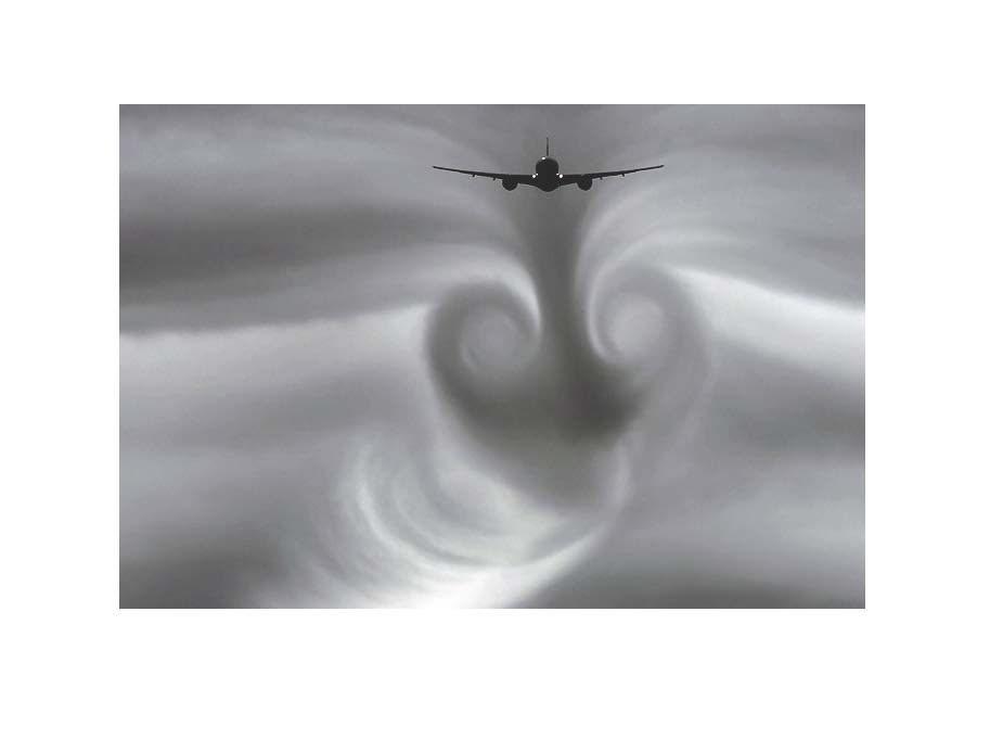
3) The Boeing analogy
This primitive (pseudo) analogy doesn’t deserve to be discussed seriously but it appears often in general media and on climate blogs so that a fast invalidation is in order. The argument takes turbulence as an example of chaos and submits that since we can design planes that fly, then the system is deterministic and chaotic dynamics are irrelevant for all practical purposes.
Here the fastest invalidation is provided by the following picture.
- CFD (computational fluid dynamics) which will solve the Navier Stokes equations with an extremely high spatial resolution
- spectral methods like von Karman which basically consider that the velocity and momentum distributions at microscopical scales are described by empirical spectral functions.
At microscopical scales and only on microscopical scales both methods (which can be further refined) give reasonable results for the purpose of computation of drag and lift so that the plane flies indeed. Yet as everybody who learned flying knows, even these models are only valid for a small range of plane velocities and attitudes. At velocities and attitudes that provoke stalling, the trajectory of the plane becomes unpredictable and chaotic and the plane no longer flies.
Both methods fail at the large space scales and are unable to predict the complex spatial structures extending behind the plane. CFD fails because the computing time scales like d^3 and there are some 7 orders of magnitude between the wing level turbulence and the large scale turbulence. The computing time is then multiplied by 10^21, which puts the numerical solving of N-S out of reach forever.
As for the spectral methods, they fail because they postulate stochastic laws for velocity and momentum distribution while the large scale structures have clearly nothing to do with randomness. If anything this picture illustrates a ‘simple’ analogy of the global attractor in that it shows how a chaotic system selects some particular spatial Fourier modes and suppresses others.
It then becomes obvious that the reasons for which planes fly and why there exists a limited computability for drag and lift on microscopical scales have absolutely no relevance for the predictability of the dynamics at larger space scales.
Symmetrically, methods that would help to describe the large scales structures would fail to understand and model the sub millimeter scales necessary to compute drag and lift.
For climate, the situation is demonstrably worse than what can be seen here because any valid climate theory has to be able to predict and explain dynamics at space scales that extend to the planetary size, e.g a further 4 orders of magnitude above the scale of the picture above.
This translates to the constraint that climate models use a resolution of O (100km) which doesn’t allow for solving N-S or any other PDE for that matter so that it is unclear what the computed numbers may represent.
4) How simple is simple ?
We have been discussing the invalidity of the most frequent analogies in the frame of fluid dynamics and more specifically in the case of Navier Stokes equations. The simplifying choice of Navier-Stokes is taken because even if the problem of turbulence and of the existence and regularity of solutions to the N-S equations is an open problem, there are still many robust results on which we can build and there are no unknown unknowns.
The first natural question to ask is how relates the complexity appearing in fluid dynamics to the complexity appearing in weather and climate.
In weather it is safe to say that the complexity is identical. Weather models are fundamentally governed by Navier Stokes only. Therefore almost everything we know about fluid dynamics can be immediately transported to weather problems.
For the climate the situation is quite different. It has been extensively analyzed in R.Pielke’s paper here. The conclusion is that by integrating the biosphere and the cryosphere, extending the time scales to centuries and the space scales to the planet, the system becomes much more complex, non linear and chaotic than the simpler weather case. Because we don’t have a theory of this more complex dynamical system that is the climate, we will restrain ourselves to the “simpler” weather case to draw some conclusions about simplicity.
As we have seen above, there exists a finite dimensional global attractor which defines the asymptotic dynamics of the system.
Considering an invariant attractor is already a first important simplification. Indeed the necessary and sufficient condition to predict the systems dynamics is to know the large number of the Fourier modes defining the global attractor. Yet the global attractor is only invariant if the coefficients (weightings) called control parameters are constant. If they vary with time because the forcings and/or the boundary conditions vary with time, then the topology and dimension of the attractor may change dramatically regardless whether the variation of the control parameters is small or large. This effect has been studied in the frame of many toy models like the Lorenz system and shows unexpected birth of new dynamical regimes for example here.
The second simplification is to try to reduce the dimension of the attractor.
One way is to use models called coupled map lattices. This paradigm treats spatio temporal chaos as a collection of N² identical chaotic oscillators situated on a NxN spatial lattice. Each oscillator is coupled to P neighbors and the dynamics of the system is then studied. The obvious limitation is that, as we have seen, the chaotic oscillator situated in Montreal is not identical to the chaotic oscillators on the pole or in Singapore. Despite the limitations of this simple model due to the variability of the local oscillators with space in the real world, it enables us to understand how complexity and spatial patterns arise when local oscillators are coupled. An excellent example how this approach is useful is here.
Another way is simply averaging spatially and/or temporally. Indeed as averaging has for effect to filter Fourier modes, it reduces the volume and the dimension of the global attractor.
However this simplification is an illusion because using an averaging operator is a one way road. Applying the averaging operator A on the global attractor Eg defines an averaged attractor Ea(A). Ea(A) has a lower dimension and a lower volume than Eg.
However for A1 ≠ A2 we have Ea(A1) ≠ Ea(A2) what destroys the universality of the averaged attractor because the topology of Ea(A) depends on the averaging operator used.
Therefore it is only possible to construct Ea(A) if Eg is known; the converse, e.g constructing Eg when Ea(A) is supposed to be known is impossible. Furthermore it is neither possible to construct Ea(A) from first principles nor to find universal metrics in which some A would be objectively privileged relative to all others.
The latter shows that the oft debated question “At what scales does the climate start ?” is meaningless.
If we classify the averaging operators Ai by the scale Si on which they average, then Si>Sj => Vol(Ea(Ai)) < Vol(Ea(Aj)). The information about the dynamics encoded in the attractor decreases monotonically when the averaging scale increases – the climate “starts” at no particular scale and the effect of averaging is to falsely decrease the variability (underestimate uncertainty) whose true value is defined only by the topology of the global attractor.
Last and third simplification is to focus on observed dominant Fourier modes and to study their dynamics, hoping that at least at shorter time scales these Fourier modes will continue to dominate. Formally this method also reduces the dimension and the volume of the attractor to a very low number. The difference to the averaging method is that the latter reduces the dimension in an arbitrary way with no justification while the former bases on evidence and doesn’t privilege any averaging scales.
Therefore this approach is superior even to the serious averaging methods. In order to avoid misunderstandings:
Here by serious averaging methods we do not mean very low dimensional deterministic models like the 1 box … N box models which belong all to the “muddling by oversimplifying” category. Indeed this category of toy models always uses a notion of equilibrium. But an equilibrium is a stable point on the global attractor and we know that the attractor contains only a large number of unstable, pseudo equilibrium points. Therefore the system’s orbit cannot be asymptotically directed towards any stable point (e.g equilibrium) because there are none.
All naïve models of the form d<T>/dt = N boxes where <T> is some spatial average of a dynamical parameter like the GMT contain no relevant information of the system’s dynamics and can be considered useless.
The dominant Fourier mode method has an advantage that we know them. ENSO is the strongest and we have an idea about its spatial and temporal Fourier modes (e.g its dimensions and pseudo periods). Follow PDO, AMO … and more generally all observed oceanic oscillations.
Tsonis, Swanson and Wyatt with the Stadium wave are examples of this approach which shows promising results. These methods have in common the choice of a finite and small number of observed dominating spatio-temporal patterns, their Fourier modes are then determined and finally one analyses how these modes interact.
5) Conclusion
The weather/climate system is arguably one of the most complex systems we know and this complexity is with us to stay. No analogy with statistical thermodynamics applies to this dissipative non equilibrium system so that an analogous simplification will not take place.
Eliminating as oversimplified and irrelevant all low dimensional deterministic toy models, the simplest approximations are probably low dimensional chaotic empirical models based on a selection of observed dominant Fourier modes and analysis of their non linear interactions (Tsonis like models). A breakthrough in coupled map lattices theory generalizing to variable local oscillators would bring us even farther.
The vulnerability of low dimensional chaotic simple models is that their predictive skills crucially depend on the validity of the founding hypothesis that the spatial and temporal Fourier modes used in the models are and stay dominating. As the time scale at which this hypothesis stays valid is unknown, the statistical predictability of the system via such models is necessarily limited in time.
JC comments: This post was submitted via email, and I did some light editing. As with all guest posts, keep your comments relevant and civil.