
by Patrick Brown
A response to Nic Lewis’ post A closer look shows global warming will not be greater than we thought.
We recently published a paper in Nature in which we leveraged observations of the Earth’s radiative energy budget to statistically constrain 21st-century climate model projections of global warming. We found that observations of the Earth’s energy budget allow us to infer generally greater central estimates of future global warming and smaller spreads about those central estimates than the raw model simulations indicate. More background on the paper can be obtained from our blog post on the research.
Last week, Nic Lewis published a critique of our work on several blogs titled A closer look shows global warming will not be greater than we thought. We welcome scientifically-grounded critiques of our work since this is the fundamental way in which science advances. In this spirit, we would like to thank Nic Lewis for his appraisal. However, we find Lewis’ central criticisms to be lacking merit. As we elaborate on below, his arguments do not undermine the findings of the study.
Brief background
Under the ‘emergent constraint’ paradigm, statistical relationships between model-simulated features of the current climate system (predictor variables), along with observations of those features, are used to constrain a predictand. In our work, the predictand is the magnitude of future global warming simulated by climate models.
We chose predictor variables that were as fundamental and comprehensive as possible while still offering the potential for a straight-forward physical connection to the magnitude of future warming. In particular, we chose the full global spatial distribution of fundamental components of Earth’s top-of-atmosphere energy budget—its outgoing (that is, reflected) shortwave radiation (OSR), outgoing longwave radiation (OLR) and net downward energy imbalance (N). We investigated three currently observable attributes of these variables—mean climatology, the magnitude of the seasonal cycle, and the magnitude of monthly variability. We chose these attributes because previous studies have indicated that behavior of the Earth’s radiative energy budget on each of these timescales can be used to infer information on fast feedbacks in the climate system. The combination of these three attributes and the three variables (OSR, OLR and N) result in a total of nine global “predictor fields”. See FAQ #3 of our previous blog post for more information on our choice of predictor variables.
We used Partial Least Squares Regression (PLSR) to relate our predictor fields to predictands of future global warming. In PLSR we can use each of the nine predictor fields individually, or we can use all nine predictor fields simultaneously (collectively). We quantified our main results with “Prediction Ratio” and “Spread Ratio” metrics. The Prediction Ratio is the ratio of our observationally-informed central estimate of warming to the previous raw model average and the Spread Ratio is the ratio of the magnitude of our constrained spread to the magnitude of the raw model spread. Prediction Ratios greater than 1 suggest greater future warming and Spread Ratios below 1 suggest a reduction in spread about the central estimate.
Lewis’ criticism
Lewis’ post expresses general skepticism of climate models and the ‘emergent constraint’ paradigm. There is much to say about both of these topics but we won’t go into them here. Instead, we will focus on Lewis’ criticism that applies specifically to our study.
We showed results associated with each of our nine predictor fields individually but we chose to emphasize the results associated with the influence of all of the predictor fields simultaneously. Lewis suggests that rather than focusing on the simultaneous predictor field, we should have focused on the results associated with the single predictor field that showed the most skill: The magnitude of the seasonal cycle in OLR. Lewis goes further to suggest that it would be useful to adjust our spatial domain in an attempt to search for an even stronger statistical relationship. Thus, Lewis is arguing that we actually undersold the strength of the constraints that we reported, not that we oversold their strength.
This is an unusual criticism for this type of analysis. Typically, criticisms in this vein would run in the opposite direction. Specifically, studies are often criticized for highlighting the single statistical relationship that appears to be the strongest while ignoring or downplaying weaker relationships that could have been discussed. Studies are correctly criticized for this tactic because the more relationships that are screened, the more likely it is that a researcher will be able to find a strong statistical association by chance, even if there is no true underlying relationship. Thus, we do not agree that it would have been more appropriate for us to highlight the results associated with the predictor field with the strongest statistical relationship (smallest Spread Ratio), rather than the results associated with the simultaneous predictor field. However, even if we were to follow this suggestion, it would not change our general conclusions regarding the magnitude of future warming.
We can use our full results, summarized in the table below (all utilizing 7 PLSR components), to look at how different choices, regarding the selection of predictor fields, would affect our conclusions.
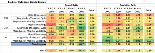
Lewis’ post makes much of the fact that highlighting the results associated with the ‘magnitude of the seasonal cycle in OLR’, rather than the simultaneous predictor field, would reduce our central estimate of future warming in RCP8.5 from +14% to +6%. This is true but it is only one, very specific example. Asking more general questions gives a better sense of the big picture:
1) What is the mean Prediction Ratio across the end-of-century RCP predictands, if we use the OLR seasonal cycle predictor field exclusively? It is 1.15, implying a 15% increase in the central estimate of warming.
2) What is the mean Prediction Ratio across the end-of-century RCP predictands, if we always use the individual predictor field that had the lowest Spread Ratio for that particular RCP (boxed values)? It is 1.13, implying a 13% increase in the central estimate of warming.
3) What is the mean Prediction Ratio across the end-of-century RCP predictands, if we just average together the results from all the individual predictor fields? It is 1.16, implying a 16% increase in the central estimate of warming.
4) What is the mean Prediction Ratio across the end-of-century RCP predictands, if we always use the simultaneous predictor field? It is 1.15, implying a 15% increase in the central estimate of warming.
One point that is worth making here is that we do not use cross-validation in the multi-model average case (the denominator of the Spread Ratio). Each model’s own value is included in the multi-model average which gives the multi-model average an inherent advantage over the cross-validated PLSR estimate. We made this choice to be extra conservative but it means that PLSR is able to provide meaningful Prediction Ratios even when the Spread Ratio is near or slightly above 1. We have shown that when we supply the PLSR procedure with random data, Spread Ratios tend to be in the range of 1.1 to 1.3 (see FAQ #7 of our previous blog post, and Extended Data Fig. 4c of the paper). Nevertheless, it may be useful to ask the following question:
5) What is the mean Prediction Ratio across the end-of-century RCP predictands, if we average together the results from only those individual predictor fields with spread ratios below 1? It is 1.15, implying a 15% increase in the central estimate of warming.
So, all five of these general methods produce about a 15% increase in the central estimate of future warming.
Lewis also suggests that our results may be sensitive to choices of standardization technique. We standardized the predictors at the level of the predictor field because we wanted to retain information on across-model differences in the spatial structure of the magnitude of predictor variables. However, we can rerun the results when everything is standardized at the grid-level and ask the same questions as above.
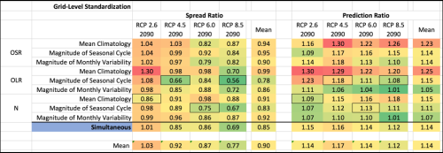
1b) What is the mean Prediction Ratio across the end-of-century RCPs if we use the OLR seasonal cycle predictor field exclusively? It is 1.15, implying a 15% increase in the central estimate of warming.
2b) What is the mean Prediction Ratio across the end-of-century RCPs if we always use the single predictor field that had the lowest Spread Ratio (boxed values)? It is 1.12, implying a 12% increase in the central estimate of warming.
3b) What is the mean Prediction Ratio across the end-of-century RCPs if we just average together the results from all the predictor fields? It is 1.14, implying a 14% increase in the central estimate of warming.
4b) What is the mean Prediction Ratio across the end-of-century RCPs if we always use the simultaneous predictor field? It is 1.14, implying a 14% increase in the central estimate of warming.
5b) What is the mean Prediction Ratio across the end-of-century RCP predictands if we average together the results from only those individual predictor fields with Spread Ratios below 1? It is 1.14, implying a 14% increase in the central estimate of warming.
Conclusion
There are several reasonable ways to summarize our results and they all imply greater future global warming in line with the values we highlighted in the paper. The only way to argue otherwise is to search out specific examples that run counter to the general results.
Appendix: Example using synthetic data
Despite the fact that our results are robust to various methodological choices, it is useful to expand upon why we used the simultaneous predictor instead of the particular predictor that happened to produce the lowest Spread Ratio on any given predictand. The general idea can be illustrated with an example using synthetic data in which the precise nature of the predictor-predictand relationships are defined ahead of time. For this purpose, I have created synthetic data with the same dimensions as the data discussed in our study and in Lewis’ blog post:
1) A synthetic predictand vector of 36 “future warming” values corresponding to imaginary output from 36 climate models. In this case, the “future warming” values are just 36 random numbers pulled from a Gaussian distribution.
2) A synthetic set of nine predictor fields (37 latitudes by 72 longitudes) associated with each of the 36 models. Each model’s nine synthetic predictor fields start with that model’s predictand value entered at every grid location. Thus, at this preliminary stage, every location in every predictor field is a perfect predictor of future warming. That is, the across-model correlation between the predictor and the “future warming” predictand is 1 and the regression slope is also 1.
The next step in creating the synthetic predictor fields is to add noise in order to obscure the predictor-predictand relationship somewhat. The first level of noise that is added is a spatially correlated field of weighing factors for each of the nine predictor maps. These weighing factor maps randomly enhance or damp the local magnitude of the map’s values (weighing factors can be positive or negative). After these weighing factors have been applied, every location for every predictor field still has a perfect across-model correlation (or perfect negative correlation) between the predictor and predictand but the regression slopes vary across space according to the magnitude of the weighing factors. The second level of noise that is added are spatially correlated fields of random numbers that are specific for each of the 9X36=324 predictor maps. At this point, everything is standardized to unit variance.
The synthetic data’s predictor-predictand relationship can be summarized in the plot below which shows the local across-model correlation coefficient (between predictor and predictand) for each of the nine predictor fields. These plots are similar to the type of thing that you would see using the real model data that we used in our study. Specifically, in both cases, there are swaths of relatively high correlations and anti-correlations with plenty of low-correlation area in between. All these predictor fields were produced the same way and the only differences arise from the two layers of random noise that were added. Thus, we know that any apparent differences between the predictor fields arose by random chance.
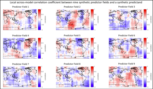
Next, we can feed this synthetic data into the same PLSR procedure that we used in our study to see what it produces. The Spread Ratios are shown in the bar graphs below. Spread Ratios are shown for each of the nine predictor fields individually as well for the case where all nine predictor fields are used simultaneously. The top plot shows results without the use of cross-validation while the bottom plot shows results with the use of cross-validation.

In the case without cross-validation, there is no guard against over-fitting. Thus, PLSR is able to utilize the many degrees of freedom in the predictor fields to create coefficients that fit predictors to the predictand exceptionally well. This is why the Spread Ratios are so small in the top bar plot. The mean Spread Ratio for the nine predictor fields in the top bar plot is 0.042, implying that the PLSR procedure was able to reduce the spread of the predictand by about 96%. Notably, using all the predictor fields simultaneously results in a three-orders-of-magnitude smaller Spread Ratio than using any of the predictor fields individually. This indicates that when there is no guard against over-fitting, much stronger relationships can be achieved by providing the PLSR procedure with more information.
However, PLSR is more than capable of over-fitting predictors to predictands and thus these small Spread Ratios are not to be taken seriously. In our work, we guard against over-fitting by using cross-validation (see FAQ #1 of our blog post). The Spread Ratios for the synthetic data using cross-validation are shown in the lower bar graph in the figure above. It is apparent that cross-validation makes a big difference. With cross-validation, the mean Spread Ratio across the nine individual predictor fields is 0.8, meaning that the average predictor field could help reduce the spread in the predictand by about 20%. Notably, a lower Spread Ratio of 0.54, is achieved when all nine predictor maps are used collectively (a 46% reduction in spread). Since there is much redundancy across the nine predictor fields, the simultaneous predictor field doesn’t increase skill very drastically but it is still better than the average of the individual predictor fields (this is a very consistent result when the entire exercise is re-run many times).
Importantly, we can even see that one particular predictor field (predictor field 2) achieved a lower Spread Ratio than the simultaneous predictor field. This brings us to the central question: Is predictor field 2 particularly special or inherently more useful as a predictor than the simultaneous predictor field? We created these nine synthetic predictor fields specifically so that they all contained roughly the same amount of information and any differences that arose, came about simply by random chance. There is an element of luck at play because the number of models (37) is small. Thus, cross-validation can produce appreciable Spread Ratio variability from predictor to predictor simply by chance. Combining the predictors reduces the Spread Ratio, but only marginally due to large redundancies in the predictors.
We apply this same logic to the results from our paper. As we stated above, our results showed that the simultaneous predictor field for the RCP 8.5 scenario shows a Spread Ratio of 0.67. Similar to the synthetic data case, eight of the nine individual predictor fields yielded Spread Ratios above this value but a single predictor field (the OLR seasonal cycle) yielded a smaller Spread Ratio. Lewis’ post argues that we should focus entirely on the OLR seasonal cycle because of this. However, just as in the synthetic data case, our interpretation is that the OLR seasonal cycle predictor may have just gotten lucky and we should not take its superior skill too seriously.

Pingback: Greater future global warming (still) predicted from Earth’s recent energy budget — Climate Etc. – NZ Conservative Coalition
Reblogged this on Climate Collections.
I think I get it… the missing heat is in the future,
Dr. Brown, I can’t discuss your article on merits because it is paywalled, but thank you for bravely wading in the lion’s den. Merry Christmas.
CG, you don’t know sci-hub? Sorry, if cry about childish paywall you are not informed enough about science to write about it. Stop it please!
Sci-hub is a pirate site that bypasses publishers by faking itself as a legitimate paid up library. Regardless of the merit of the publishers’ rights, I scarcely think judging someone as a scientist based on their knowledge about how to pirate is warranted or appropriate.
Yup “failure to pirate” is not much of an argument. Except for progressives…. for whom following tbe law always seems irrelevant.
His original blog on the Nature paper, which has been linked, and videos there explain it well enough.
So, validating a complex model with many moving parts and variables with a system that is likewise complicated is difficult. But if we can both calculate and measure the earth’s energy budget, can’t things be simpler? I mean if we know how much the energy leaving the planet is decreasing don’t we then know how the vertical temperature of our atmosphere is increasing? A simple two-dimensional model will have all of the effects of forcings and feedbacks built-in. Decrease in energy leaving equals increase due to greenhouse gasses, to a close approximation. Is this way too simple?
That’s essentially what Arrhenius did over a century ago. It remains basically correct to first order.
jim Yes I think it is too simple. As CO2 and temperatures are increasing there is little change in Outgoing Longwave Radiation. It seems to be increasing a little bit. So greenhouse gases are cooling the climate at Top Of Atmosphere, and for the earth at whole. It is the Short Wave Radiation that heats the world, by radiating less to space. The redistribution of heat that LWR (and Greenhouse gases) has, has some effect at the surface.
This is the reason I keep asking about how the models represent this, and the reason that surface temperature speculations are of less interest.
So I will ask again: Which models are best to predict surface temperatures in 2090 according to Brown? What change do these models show for OLR?
What are the error bars around the three energy budget datasets? I suspect they are quite large. Even if known quite well, however, how long might it take before a net downward energy imbalance has an effect on global temperature? 1000 years, to account for ocean overturning?
An effect on global surface temperature comes first.
Then, the surface air being warmer than the surface ocean waters, the surface ocean layers start to warm.
Then, gradually, the surface waters are mixed in to the deeper waters.
So the air can get a fair bit ahead of the deep ocean, particularly as it’s really the surface ocean layers that mainly slow down the atmospheric warming, not the deep ocean.
The slower the rate of ocean overturning, the faster the early surface warming. Think of it: the more often those cold waters come up and mix with the surface layers, the longer it would take to get the surface layers’ temps up.
In contrast, if the waters are stagnant, the surface water temps can more easily warm up with the atmosphere. The effective short-term heat sink that the atmosphere has to heat up is smaller.
Kudos to Patrick Brown for showing up here and responding, in a thoughtful and polite manner. This is how science should be done.
Agreed, Patrick brown should be congratulated for defending his ground.
Let’s hope Nic Lewis does the same and they can have a meaningful and polite scientific debate.
Tonyb
And soft unstable ground it is to defend.
Models all the way down.
/shrug. All science is models.
That’s the point – to build models of how the world works, which can be as simple as Newton’s law of gravitation or as complex as a full model of protein interactions in the human body.
A “model” is just a descriptor of how something works.
Dr Brown,
Also thanks and we appreciate your thoughtful response and courteous discussion. This is science at it’s enlightened best.
scott
Patrick, Since you are here, I would like your reaction to this observation from Mauretsen and Stevens:
Maybe I got it wrong, but my understanding is thar Brown and Caldeira looked for the most skillful models for the years from 2001 to 2015, and the components of TOA radiation were the only variables.
In that paper they go on to say, bold mine:
I believe Brown and Caldeira used the model mentioned, MPI-ESM-LR, in their study.
JCH, That’s irrelevant to my point which is that if they had chosen aerosol forcing (which is emergent in many GCM’s) their result would have been the opposite. In any case, a more severe criticism of this work is just the general lack of skill of GCM’s generally and the very crude models of many of the sub grid processes. Another interesting exchange comes from a group of climate modelers attempting to use GCM’s to show that aerosol forcings are indeed more negative than Stevens claimed based on data. Here’s a quote from Steven’s response:
I like the part about “the fantasy.”
The OSR magnitude and pattern would be affected by aerosols, so that would have been included in the skill measure, but only to the extent that it matters for the energy budget.
“Atmospheric and oceanic computational simulation models often successfully depict chaotic space–time patterns, flow phenomena, dynamical balances, and equilibrium distributions that mimic nature. This success is accomplished through necessary but nonunique choices for discrete algorithms, parameterizations, and coupled contributing processes that introduce structural instability into the model. Therefore, we should expect a degree of irreducible imprecision in quantitative correspondences with nature, even with plausibly formulated models and careful calibration (tuning) to several empirical measures. Where precision is an issue (e.g., in a climate forecast), only simulation ensembles made across systematically designed model families allow an estimate of the level of relevant irreducible imprecision.” http://www.pnas.org/content/104/21/8709.full
Wonder which blog JCH found that on. A paper on tuning a model claims that the model isn’t tuned? And someone selectively quotes because it accords with motivated reasoning. Then JCH imagines it is a definitive point and repeats it here. Ratbag nonsense as usual.
Tuned verisimilitude – btw – is not a measure of skill – nor can it guarantee future verisimilitude.
I don´t get how: “observations of the Earth’s energy budget allow us to infer generally greater central estimates of future global warming”
The central estimate for current total feedback from clouds provided by IPCC was 0.6 W/m². (2013)
(ref.: AR5; WGI; Figure 7.10 | Cloud feedback parameters; Page 588)
The central estimate for global accumulation of energy was also 0.6 W/m²: (2013)
«considering a global heat storage of 0.6 W/m²»
(ref.: AR5; WGI; 2.3.1 Global Mean Radiation Budget; Page 181)
Simple arithmetic tells me that if one term on one side of an equality sign is equal to one term on the other side of an equality sign, then the sum of all other terms in that equality, including radiative forcing from CO2, must be zero. Which is not in accordance with the propounded theory.
This indicates to me that either the central estimate for the cloud feedback effect or the estimated effect from CO2 must have been overestimated by IPCC.
I don´t get how a greater central estimate for future global warming can be inferred from an energy budget that indicates that either the cloud feedback effect or the radiative forcing from CO2, or both, seems to be lower than estimated by IPCC.
The cloud feedback was given as 0.6W/m2/degree C. It is additive to greenhouse forcing and there is a broad range given.
From figure 7.10 the central estimate for the cloud feedback parameter from CMIP5 models that IPCC rely on seems to be about 0,65W/(m2*DegC), where DegC is the warming since pre-industrial times. The central estimate for warming since preindustrial times is provided by IPCC as 0,85 DegC. Ref. page 5 in the same report.
0,65 W/(m2*DegC)*0,85 DegC = 0,5525 W/m2
I rounded the result to 0,6 W/m2.
There is no statistically meaningful central estimate – this is after all the subject of the post. And half that warming was quite natural.
But there are other sources of cloud variability.
“Marine stratocumulus cloud decks forming over dark, oceans are regarded as the reflectors of the atmosphere.1 The decks of low clouds 1000s of km in scale reflect back to space a significant portion of the direct solar radiation
and therefore dramatically increase the local albedo of areas otherwise characterized by dark oceans below.2,3 This cloud system has been shown to have two stable states: open and
closed cells. Closed cell cloud systems have high cloud fraction and are usually shallower, while open cells have low cloud fraction and form thicker clouds mostly over the convective
cell walls and therefore have a smaller domain average albedo.4–6 Closed cells tend to be associated with the eastern part of the subtropical oceans, forming over cold water (upwelling areas) and within a low, stable atmospheric marine boundary layer (MBL), while open cells tend to form over warmer water with a deeper MBL.” http://aip.scitation.org/doi/pdf/10.1063/1.4973593
Yes – the cloud feedback is additive to greenhouse forcing, that is one of my main points.
The hypothezised cloud feedback effect is a direct response to atmospheric warming and not a direct response to the increase in CO2 levels in the atmosphere.
As Robert points at, a feedback is extra energy accumulation for a given amount of warming. This may have been on past warming, present warming, or be future warming, whatever. “For X degrees of temperature change from other causes, we expect Y amount of additional feedback”.
The present global accumulation of energy is simply the present accumulation of energy.
The two aren’t comparable. The feedback is *on* some amount of warming, incrementally. It’s not like 1 degree of warming happens from CO2, and then, and only then, the feedback kicks in. No, it’s happening all along.
Meanwhile, the global accumulation of energy just relates to how much warming we have left to go. Since we’ve already warmed somewhat, it is necessarily true that the amount of forcing+feedback left from the CO2 that we’ve emitted thus far is less than the total.
Ex: We emit enough CO2 to cause 1 W/m2 in forcing, and an additional 2 W/m2 in feedbacks. 3 W/m2 total.
The Earth warms for a while. Now we hit a point where the energy accumulation is 0.5 W/m2. What does this tell you about feedbacks? Not much, as the warming isn’t finished, so the feedbacks haven’t finished kicking in.
You can’t compare the feedbacks we’ll have for a given amount of warming to the present energy accumulation. It’s apples and giraffes.
Dang it, wish I could edit that.
That example is 3 W/m2 at equilibrium.
That’s the key point. The CO2 forcing starts right away, but the feedbacks don’t; their numbers are for equilibrium (or for a given amount of warming; which works out to the same thing).
It is assumed that net feedbacks are negative – otherwise there would be additional warming and therefore additional feedbacks in an unstable loop. The Planck feedback is non-linear and increases to the fourth power with temperature keeping things on an even keel.
http://www.azimuthproject.org/azimuth/show/Climate+forcing+and+feedback
Feedbacks to atmospheric warming are quick. Some believe that the ocean is slow to equilibriate leading to slow feedbacks. Others that ocean equilibrium occurs more rapidly. I’m in the latter camp. Oceans cool to equilibrium at the very least on an annual basis rather than warm slowly.
Sorry for no reply, morning now, and workday ahead.
whateva…
The reason the imbalance is less than the GHG forcing so far, which exceeds 2 W/m2 is that the rest is canceled by the warming we have already had. As I have been saying, all the warming we have had in response to GHGs is still not enough to cancel all the forcing, which is important for the attribution argument, because this logically implies >100% attribution due to the remaining imbalance. Skeptics poorly understand this point about the observational evidence.The positive imbalance means we have not caught up with the forcing change that is also ongoing.
A lot of this and Nick Lewis’ recommendations are basically p-hacking and thus subject to false outcomes
Cryptic as always Eli. P-hacking indeed. The key is this: “It is always worse than we thought.” You may want to have that tattooed on your forehead. As time passes, your tatoo will become ever more humorous.
“Data dredging (also data fishing, data snooping, and p-hacking) is the use of data mining to uncover patterns in data that can be presented as statistically significant, without first devising a specific hypothesis as to the underlying causality.”
there is going to be future global cooling which is now starting.
I’ve been reading WUWT since the early 00’s, and every year, the cooling has been just around the corner.
Annnnnny day now. I’m sure it’s coming. Just you wait.
For “any day now” predictions that never come, it’s right up there with the second coming of Christ and the coming global financial collapse.
Let’s not gloss over model deficiencies.
“The top-of-atmosphere (TOA) Earth radiation budget (ERB) is determined from the difference between how much energy is absorbed and emitted by the planet. Climate forcing results in an imbalance in the TOA radiation budget that has direct implications for global climate, but the large natural variability in the Earth’s radiation budget due to fluctuations in atmospheric and ocean dynamics complicates this picture.” https://link.springer.com/article/10.1007/s10712-012-9175-1
Over the short term – say 2001 to 2015 – changes in the emitted IR and reflected SW are dominated by secular changes in cloud, ice, vegetation and dust emerging from ocean and atmospheric circulation. The Earth flow field is turbulent and chaotic and Hurst effects emerge in both space and time. How this will change in the future is not knowable. The math and physics for this are as yet primitive compared to the complexity of the problem. What an admission that would be.
Nor is the radiative imbalance obtainable from toa measurements but is derived from that dubious assumption that short term and very complex ocean heat changes are the result exclusively of greenhouse gases. Tuning to this derived parameter is grossly simplistic.
Nor is a model itself anything less than chaos. Not just two non-unique solutions for each model but potentially many 1000’s. The nature of opportunistic ensembles such as CMIP5 is a collection of solutions arbitrarily selected from a broad range.
http://www.pnas.org/content/104/21/8709/F1.large.jpg
This has been known for 50 plus years. Do they really not know or is it a conspiracy of ignorance from a cultural bias? Either way it is all just appalling nonsense.
So we have models in which the physics are inadequate, that evolve with substantial variability – indeed with Hurst effects – from nonlinear core equations of fluid transport and that are tuned to poorly constrained parameters. Redeeming existing models for the purpose of century scale climate prediction is a lost cause. What would be needed first is better physics, better observations and massively more computing power to reduce the grid size. This would reduce the irreducible imprecision (the spread of the solution space) of any particular model. Moreover the real world will continue to diverge chaotically from chaotic models.
Just because something simplistic can be done – doesn’t mean that it ought to be – or that is provides light on the subject. This study is building on sand and as such is very poor science in a field already replete with very poor science.
Let’s give the figure caption.
“Generic behaviors for chaotic dynamical systems with dependent variables ξ(t) and η(t). (Left) Sensitive dependence. Small changes in initial or boundary conditions imply limited predictability with (Lyapunov) exponential growth in phase differences. (Right) Structural instability. Small changes in model formulation alter the long-time probability distribution function (PDF) (i.e., the attractor).” http://www.pnas.org/content/104/21/8709.full
There are two things possible with models. A probability distribution function on individual model ‘irreducible imprecision’ – the entire chaotic solution space for any model. Or initialized decadal forecasts with nested regional downscaling at finer scales and ocean sea surface temperature coupling. Both have immense and unresolved theoretical and practical problems. Who can afford the computing power or the electricity bill. Tim Palmer has suggested ‘inexact computing’ – just like the human brain. Some of us are better at that than others.
“our results showed that the simultaneous predictor field for the RCP 8.5 scenario shows a Spread Ratio of 0.67”
.
Hmmm….
RPC 8.5 is wildly disconnected from reality. How about other more realistic RPC’s?
I any case, it would be much more credible to look at the individual model projections against measured reality, and reject those models which are clearly deficient.
Yes, any study that uses RCP 8.5 can be dismissed out of hand for unrealistic. It is an extreme scenario that cannot take place.
It is certainly a good sign that the measured satellite data is being used in the analysis. It’s been a while since I looked at ERB data (pre-2000) but I’ll have a look. I appreciate the civil discussion.
t is interesting to see how scientists now are jumping off the bandwagon. Allen, Forster and other prominent scientists say “It is better than we thougt”, while Brown and others are clinging to their run-away-train.
https://www.nature.com/articles/ngeo3031?foxtrotcallback=true
It is a noticeable shift for the skeptics that they now favor papers like this that call for “strengthening near-term emissions reductions”. We didn’t used to see this so much, but it is a promising trend for them to finally support such programs.
Jim D: I think the 1,5 deg limit is far to low. It was partly based on a bluff from Hansen et ,al. which was released to the Paris conference. Caldeira was one of his puppets in this mission.So if we still should have the 2 deg as a limit, we would have plenty of time.
From climate researcher Glen Peters:
“The implications of this paper are breath taking. No, I am not exaggerating. And the implications are to do both with politics and with science.
For politics, the stakes are high. Just ponder these two potential outcomes:
Suppose the paper is correct, then 1.5°C is a distinct possibility, about the same effort that we previously thought for 2°C. There would be real and tangible hope for small island states and other vulnerable communities. And 2°C would be a rather feasible and realistic option, meaning that I would have to go eat some serious humble pie.
Suppose we start to act on their larger budgets, but after another 5-10 years we discover they were wrong. Then we may have completely blown any chance of 1.5°C or 2°C.
I seriously hope they have this right, or at least, I hope they will be vocal if they revise their estimates downwards!
For science, I can’t help but frame the paper in two ways:
We understand the climate system, but a more careful accounting shows the carbon budgets are much larger.
We don’t understand the climate system.”
“On the first point, I already have serious reservations with the IPCC carbon budgets, mainly because of uncountable inconsistencies. Since the authors modify something I don’t really trust in the first place, then I am a little cautious of the findings. But, if the climate system behaves as we thought, then careful accounting should allow us to reconcile the difference between the original and updated carbon budgets. Science has made progress.
On the second point, the paper is going to have ripple effects. If their adjustments are correct, then those adjustments may cause inconsistencies elsewhere. Do we have the climate sensitivity wrong? Some argue that committed warming and aerosols would push us over 1.5°C. My mind boggles at the potential implications if the second point is realised.
Because of the political and scientific implications of this paper are so immense, it will need a rigorous assessment by the scientific and policy communities. That is going to take time, perhaps years.”
Ref. https://www.carbonbrief.org/guest-post-why-the-one-point-five-warming-limit-is-not-yet-a-geophysical-impossibility
I don’t believe in all this fine-tuning of targets. The first order of business is to bend the global emissions curve downwards as soon as possible and work from there. China is the main problem in that regard.
Sorry. It was the 2 deg limit that were based on Hansen et al paper.
I have explained the bluff at SoD.
https://scienceofdoom.com/2017/06/25/the-confirmation-bias-a-feature-not-a-bug/#comment-119101
I`m sorry Caldeira, for bringing up a close tie to Hansen. My memory failed me. I thought you were one of those who were into the mission of Juliana lawsuit against United States, and extracting CO2 from the atmosphere. As I also commented ar SoD.
https://scienceofdoom.com/2017/06/25/the-confirmation-bias-a-feature-not-a-bug/#comment-120089
You can do Kalman filtering to get the best values for everything in sight from the data. It’s especially suited to updating with new data and giving you the best model parameter updates and prediction updates.
It amounts to weighted least squares but in a recursive form that’s handy.
It also makes obvious what you’re doing, which regular statistical forms don’t do.
In particular, if the model is no good, the result is no good, as you can see with a simple thought experiment in the recursive form.
(Kalman filtering is used for tracking stuff mostly but works anywhere least squares makes sense.)
It is annoying that Patrick Brown has posted a technical argument here and seems to be ignoring any questions or discussion.
It’s Christmas.
Not having read in depth either the Brown paper or the Nic Lewis and Brown threads posted here, I will limit my comments to some questions that arise from some comparisons I have made for CMIP5 model derived climate variables to those from observation during the historical period. I have also compared individual climate models to one another.
In my analyses I have used the variables of global mean surface temperatures (GMST) over various periods of time, the ratio of Northern versus Southern hemisphere warming, the amount of red and white noise in the GMST series, and presence of reoccurring cyclical structure in the GMST series. I have used the surface temperatures for land and the SST for the oceans in these analyses such that I have an oranges to oranges comparison.
I also limited my analyses to comparing an individual climate model series to the observed series and then only when the climate model had multiple runs. The comparison here can only be made with reference to where the observed series falls on the probability distribution of the climate model multiple runs. I never statistically lump all the climate series together but rather treat the individual series as independent from one another. I also realize and statistically treat the observed series as a single realization of a chaotic system. In comparison thus with climate model versus climate model and climate model versus observed requires one the pairs to be a climate model with multiple runs – and the more runs the better.
Finally the TOA energy balance (no creation or destruction of energy allowed) is not generally well maintained in the CMIP5 models and the drifting and trending in the pre-industrial runs is difficult to apply as a compensating factor for the energy imbalance.
Questions to the Brown paper authors or others who might have the background information to answer these questions:
1. Was the energy balance described above noted or considered in the selection or weighting of the models?
2. Were the climate models considered as an ensemble with at least some dependence or as independent?
3. Were there any sensitivity tests using other metrics outside of the TOA metrics mentioned here? [For example, how believable would be the results from a model – with multiple runs – that had good agreement with the observed on the global TOA metrics but put the observed NH/SH warming ratio, for surface (or TOA metrics, for that matter) far into the tail of the multiple probability distribution].
A final comment would be how confident are we and the Brown paper authors that the model results for the historical period are from near first principles and not so much from in-sample modeling that we can have good confidence in the out-of-sample results following the modeled predictions.
Judith : Is it not true that the harsh reality is that the output of the climate models which the IPCC relies on for their dangerous global warming forecasts have no necessary connection to reality because of their structural inadequacies. See Section 1 at
https://climatesense-norpag.blogspot.com/2017/02/the-coming-cooling-usefully-accurate_17.html
Here is a quote:
“The climate model forecasts, on which the entire Catastrophic Anthropogenic Global Warming meme rests, are structured with no regard to the natural 60+/- year and, more importantly, 1,000 year periodicities that are so obvious in the temperature record. The modelers approach is simply a scientific disaster and lacks even average commonsense. It is exactly like taking the temperature trend from, say, February to July and projecting it ahead linearly for 20 years beyond an inversion point. The models are generally back-tuned for less than 150 years when the relevant time scale is millennial. The radiative forcings shown in Fig. 1 reflect the past assumptions. The IPCC future temperature projections depend in addition on the Representative Concentration Pathways (RCPs) chosen for analysis. The RCPs depend on highly speculative scenarios, principally population and energy source and price forecasts, dreamt up by sundry sources. The cost/benefit analysis of actions taken to limit CO2 levels depends on the discount rate used and allowances made, if any, for the positive future positive economic effects of CO2 production on agriculture and of fossil fuel based energy production. The structural uncertainties inherent in this phase of the temperature projections are clearly so large, especially when added to the uncertainties of the science already discussed, that the outcomes provide no basis for action or even rational discussion by government policymakers. The IPCC range of ECS estimates reflects merely the predilections of the modellers – a classic case of “Weapons of Math Destruction” (6).
Harrison and Stainforth 2009 say (7): “Reductionism argues that deterministic approaches to science and positivist views of causation are the appropriate methodologies for exploring complex, multivariate systems where the behavior of a complex system can be deduced from the fundamental reductionist understanding. Rather, large complex systems may be better understood, and perhaps only understood, in terms of observed, emergent behavior. The practical implication is that there exist system behaviors and structures that are not amenable to explanation or prediction by reductionist methodologies. The search for objective constraints with which to reduce the uncertainty in regional predictions has proven elusive. The problem of equifinality ……. that different model structures and different parameter sets of a model can produce similar observed behavior of the system under study – has rarely been addressed.” A new forecasting paradigm is required.
Here is an abstract of the linked paper:
norpag@att.net
DOI: 10.1177/0958305X16686488
Energy & Environment
“The coming cooling: usefully accurate climate forecasting for policy makers
ABSTRACT
This paper argues that the methods used by the establishment climate science community are not fit for purpose and that a new forecasting paradigm should be adopted. Earth’s climate is the result of resonances and beats between various quasi-cyclic processes of varying wavelengths. It is not possible to forecast the future unless we have a good understanding of where the earth is in time in relation to the current phases of those different interacting natural quasi periodicities. Evidence is presented specifying the timing and amplitude of the natural 60+/- year and, more importantly, 1,000 year periodicities (observed emergent behaviors) that are so obvious in the temperature record. Data related to the solar climate driver is discussed and the solar cycle 22 low in the neutron count (high solar activity) in 1991 is identified as a solar activity millennial peak and correlated with the millennial peak -inversion point – in the UAH temperature trend in about 2003. The cyclic trends are projected forward and predict a probable general temperature decline in the coming decades and centuries. Estimates of the timing and amplitude of the coming cooling are made. If the real climate outcomes follow a trend which approaches the near term forecasts of this working hypothesis, the divergence between the IPCC forecasts and those projected by this paper will be so large by 2021 as to make the current, supposedly actionable, level of confidence in the IPCC forecasts untenable.”
Pingback: Reply to Patrick Brown’s response to my article commenting on his Nature paper « Climate Audit
At a basic, empirical level : if indeed we can measure the radiation budget at TOA in absolute terms, can we not just map this against C02 levels and so settle the whole matter ? And why too then the recourse to complex models ?
I have replied to this article at https://climateaudit.org/2017/12/23/reply-to-patrick-browns-response-to-my-article-commenting-on-his-nature-paper/
Pingback: Weekly Climate and Energy News Roundup #297 | Watts Up With That?
Pingback: Reply to Patrick Brown’s response to comments on his Nature article | Climate Etc.
Pingback: Reply to Patrick Brown’s response to my article commenting on his Nature paper | Watts Up With That?
There is no point in discussing the paper, since it is not open access.
https://www.nature.com/articles/nature24672
That said, Earth’s radiative energy budget is not observed, systematic error in CERES ToA all sky absorbed shortwave vs. outgoing longwave is far too large for that.
https://ceres.larc.nasa.gov/order_data.php
EBAF-TOA
Monthly and climatological averages of TOA clear-sky (spatially complete) fluxes, all-sky fluxes and clouds, and cloud radiative effect (CRE), where the TOA net flux is constrained to the ocean heat storage.
“The CERES EBAF-TOA product was designed for climate modelers that need a net imbalance constrained to the ocean heat storage term”
“The CERES absolute instrument calibration currently does not have zero net balance and must be adjusted to balance the Earth’s energy budget.”
So. It is not NET ToA radiative imbalance which is measured, but ocean heat storage.
It is measured by ARGO floats (down to a depth of 2000 m, since 2007), but too many assumptions go into it to be taken as definitive.
Therefore it can “statistically constrain” nothing and I don’t even know why radiative energy budget is mentioned.
The point is, if ARGO is to be believed, average temperature of oceans down to a depth of 2000 m has increased by some 0.03°C in the last 10 years. Which is important why? And how ARGO is supposed to detect an annual change of 0.003°C? Which is about the accuracy of thermometers in ARGO floats (± 0.002°C). And then, sensor drift and thermal lag is not even taken into account. These are corrected by expert examination at a later stage, a huge no-no in science.
“…corrected by expert examination at a later stage, a huge no-no in science…”
Shhhhhh! You’re talking about the life’s blood of the cause here.