
by Steve McGee
In science, one likes to have more examples than theories. – Dusan Djuric
Those words, spoken whimsically about cosmology, apply to climate science as well. The theory of the sensitivity of climate to the radiative forcing imposed by a doubling of carbon dioxide suffers from a lack of observed, repeatable examples. Paleo-climate studies carry with them the uncertainty of the proxy data and unmeasured assumptions on which they are based. Studies regarding the forcing from volcanoes and other transient events may not be repeatable for some time. However, Lindzen et. al. 1995 (link ) and Ramanathan and Inamdar in Frontiers of Climate Modeling, 2006 (link ) each have pointed out that the seasonal variation of earth temperature is quite large and possibly a surrogate for climate change. With this in mind, I set out to determine how the seasonal variation occurred in the CFSR data set ( described at this link, and data available at this link ), which I examined in a previous post Is earth in energy deficit? Because of some missing data, the following analyses exclude all observations from the year 1994.
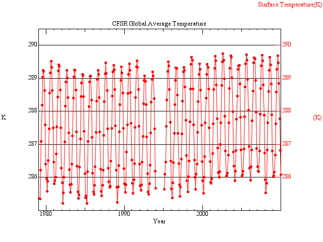
The global average temperature variation, below, does indeed reflect a large signal. As described in the references, this variation stems from the fact that land has a much lower heat capacity than the oceans and that most of the earth’s land surface exists in the Northern Hemisphere. This arrangement amplifies the effect of the Northern Hemisphere seasonal cycle and dampens the effect of the Southern Hemisphere seasonal cycle in the global mean surface temperature.
We can see this pattern more clearly in the global averages by month. Not only does the surface temperature vary, but so too does the outgoing longwave radiation.

Precipitable water is an absolute measure of water vapor in the atmosphere which also co-varies with surface temperature. This is consistent with water vapor feedback.

A correlation of all outgoing radiance versus temperature for all months yields the following plot. The darker shaded area represents a variance within 1 standard deviation. The lighter shaded area represents a variance within 2 standard deviations.

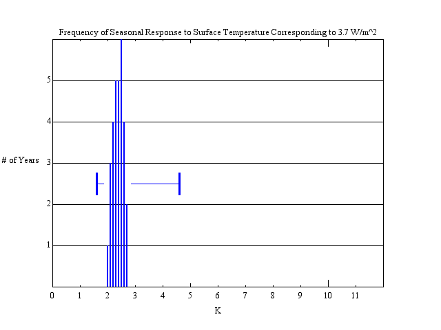
Each year of response becomes an individual example or experiment in how earth emits longwave radiation in response to surface temperature change. And by collating the number of years that the correlated response falls into specific ranges, we arrive at a rough indication of the frequency. Dividing 3.7 W/m^2, which is the assumed value of radiative forcing for a doubling of carbon dioxide, by the observed seasonal correlation of energy and temperature, results in the analogous temperature response. The error range indicated ( 1.6C to 4.6C ) is that of all the monthly data considered. The range of annual observed seasonal correlations is from 2.0C to 2.7C. The most frequent correlated response for the CFSR years was 2.5C.
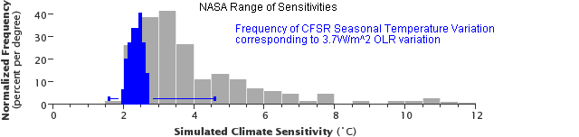
By overlaying the CFSR seasonal response frequency over the chart ( at this link ) we can compare the seasonal response to the sensitivities indicated by climate models. ( the scale for seasonal response remains in years, not normalized frequency ).
Strengths and Weaknesses of this approach
There are number of strengths and weaknesses to using the seasonal response as an analog to climate change induced by greenhouse gasses. Strengths include: 1.) The large range of outgoing longwave radiation is around 6 W/m^2 which is considerably larger than the 3.7W/m^2 estimated to result from carbon dioxide doubling. 2.) The variation in the global mean, not just smaller regions. 3.) The repeatability of each year’s variation which creates a new example of radiative response 4.) The water vapor feedback and all other fast feedbacks are included in the variation.
Weaknesses include: 1.) The uncertainty inherent in re-analyses data set. However, one of the largest sources of error in re-analyses is the change in instruments which can introduce longer term trends. But because the seasonal data compares the averages per month, potential changes in data sets are smoothed. 2.) No shortwave feedbacks are included by examining only the seasonal OLR response to surface temperature while the climate models do include albedo feedback. This is lessened somewhat by recalling that albedo feedback is estimated to be the weakest feedback ( see Soden and Held at this link ). 3.) Perhaps most importantly, the very assymetry that produces the temperature fluctuation produces different patterns and distributions of temperature, jet streams, ITCZ, tropopause heights, and a many of other dynamic features of the atmosphere. The change from radiative forcing, from lesser forcing to greater forcing, integrated year round is a different distribution of response than the seasonal change we examine here from winter to summer and back to winter. These questions are beyond this look at the data, but would seem worth pursuing. It should also be pointed out that paleo-climate also has a different distribution than present climate – miles high ice-sheets where plains lie today, lower sea level, and so on.
Comments
There is much to consider here. Climate sensitivity is usually assessed with temperature as the dependent variable: ‘How much will surface temperature rise in response to a given radiative forcing?’ The meaning of the seasonal response is that outgoing longwave radiance is the dependent variable: ‘How much will outgoing radiance rise in response to surface temperature rising?’ In the longer term, these relationships are the same, for if a radiative forcing is imposed, heat will accumulate and raise the surface temperature which increases the OLR to the level at which heat accumulation stops.
The precipitable water values are not used in the simple correlation above, but I included the plot as a reminder that water vapor does appear to provide a feedback. The fact that the implied seasonal sensitivity of 0.65C per W/m^2 is greater than the Planck response indicates a net positive feedback. It is sometimes expressed that global warming will accelerate because positive feedbacks are lagging. The evidence in the seasonal response is that the largest identified feedback, water vapor, responds within a month – a fast feedback indeed.
In some ways, the seasonal response confirms current understanding of climate sensitivity. Hansen et. al. 2013 ( at this link ) find a paleo-climate sensitivity of 0.75C per W/m^2. The reciprocal of the observed seasonal correlation above yields 0.65C per W/m^2. And the range of uncertainty in the seasonal response ( 1.6C to 4.6C ) is quite similar to those suggested by the IPCC. On the other hand, the frequency of years of best seasonal correlation indicate a much less variable range than many models do for future climate. Further, the seasonal responses do not support the higher sensitivities indicated by some model runs.
Ultimately, Lindzen decided that the seasonal variation was not a ‘surrogate’ for ‘climate change’ within the constraints of the data set he was using. Perhaps ‘analog’ is a better description. The morphology of the variations are clearly different, but the strong global average variation and expected features make the seasonal response an important phenomenon worth further study.
Biosketch: Steve McGee has a bachelor of science degree in meteorology. His long career of software engineering includes the development of numerous defense related systems providing analysis and display weather and atmospheric effects. Steve’s previous post at Climate Etc.:
JC comment: This post was submitted via email. As with all guest posts, please keep your comments relevant and civil.

It all comes down to personal responsibility. We able to create whimsical views of the world so quickly that, depending on our motives if predicting problems, we can always be a step ahead of a reasoned analysis of how serious such ‘problems’ really are.
Waggy, you have me scratching my hand. I can’t figure out whether you are
a. agreeing with Steve McGee
b. disagreeing with Steve McGee
or
c. just wanted to say something irrelevant
Make that “scratching my head” rather than “scratching my hand.” I do know the difference.
Restricting knowledge by using a computer to make the world obscure …
You believe Steve McGee is “restricting knowledge by using a computer to make the world obscure …”
It’s not nice to imply guest poster Steve is crooked. Perhaps you forgot what our hostess Judith Curry said. ” As with all guest posts, please keep your comments relevant and civil.”
Climate alarmists essentially are unintelligible because they do not want to be understood. The climate ‘experts’ of AGW theory take every opportunity to lecture us on our limitations by telling all of us that only other government climatists are capable of understanding the ‘science’ of climate change.
Max_OK there are over the counter meds you can get to reduce the urge to scratch different body parts and if those aren’t effective your doctor can prescribe stronger things.
Did the increase in temperature causing the T4 increase in longwave emission occur at the ocean surface, land surface, low latitudes, high latitudes, or from tops of clouds? Where the temperature increase is happening is at least as important and how much if not moreso. In the winter in higher latitudes people welcome warming. If the increase is from a more active water cycle which is insensibly transporting the extra energy from the surface to cloud tops sparing the ocean and/or land surface the rise in temperature who would care since we don’t live or work at the level of cloud tops?
The surface temperature is the global average ( land and ocean surface ).
As you point out, very little of the outgoing longwave is emitted directly from the surface – the large majority coming from clouds and water vapor aloft. But also as you point out, the surface is the prime human habitat, and indeed, the surface temperature and outgoing longwave correlate very well.
…the surface temperature and outgoing longwave correlate very well.
http://s1114.photobucket.com/user/Chief_Hydrologist/media/HadCRUT4vCERES_zpse5107cfd.png.html?sort=3&o=5
I’m not familiar with the CFSR data set. What instruments determine the global average temperature and what instruments measure outgoing longwave radiation in this CFSR data set?
Global average temperature graphs in the OP begins ~1979 so I’m assuming it’s satellite data. RSS or UAH? I’ve never seen absolute temperature given in Kelvin so that’s a red flag right there. Absolute average surface temperature of the earth is a controversial number and as such is always referred to as an anomaly from a baseline.
Since the conclusions can be no more reliable than the data I really can’t take this seriously without knowing more about the data source(s).
The CFSR would get the radiation from the model atmospheric variables. It is not an observation, but an inference with a radiative model.
Steve McGee | December 26, 2013 at 2:51 pm |
“But also as you point out, the surface is the prime human habitat, and indeed, the surface temperature and outgoing longwave correlate very well.”
Not really. I see numerous departures of polar opposite polarity in the short (since 2000) HadCRUTR4 vs. CERES graph that Chief Hydrologist was kind enough to provide. Correlation does not equal causation of course but the correlation between sunspot count and surface temperature is compelling as well. Outgoing radiation across the planet is notoriously difficult to measure because it goes out in all directions and we don’t have a million satellites monitoring it everywhere at once. Incoming radiation is a cinch in comparison because it’s a point source (the sun) and even that is controversial in accuracy and precision because of instrumentation degradation and drift when it comes down changes on the order of single watts or less per square meter. This is the bane of climate science in general. The instruments we have are not nearly good enough to tease out such small numbers and that is precisely why I must know more about the hardware and data processing before establishing some level of trust in the dataset. There is WAY too much room for mischief in trying to improve data from hardware that simply isn’t up to the tasks being asked of it.
David Springer, “Global average temperature graphs in the OP begins ~1979 so I’m assuming it’s satellite data. RSS or UAH? I’ve never seen absolute temperature given in Kelvin so that’s a red flag right there. Absolute average surface temperature of the earth is a controversial number and as such is always referred to as an anomaly from a baseline.”
That is a bit odd. You can get SST and lower troposphere in absolute, but “global” surface?
Springer its reanalysis as the article points out. You dont have the chops to question it. Out of your league again.
Comparisons between CERES Terra and Aqua for July 2002–February 2010 (Table – 1) show SW ‘‘trend’’ consistency of 0.04 ± 0.27 Wm^2 in the tropics and 0.12 ± 0.25 Wm^2 for the globe. In the LW, differences are much larger: the Terra minus Aqua difference is -0.39 ± 0.21 Wm^2 for 30S–30N, and for the globe, it is 0.63 ± 0.36 Wm^2. http://meteora.ucsd.edu/~jnorris/reprints/Loeb_et_al_ISSI_Surv_Geophys_2012.pdf
CERES trends are especially accurate in SW.
http://www.youtube.com/watch?v=MGR-QGw7Mr8
The correlation of CERES and HadCRUT4 graph I showed is 0.21. I am sure I could get better with some lag – but there are all sorts of complexities and feedbacks such that a 1 to 1 correspondence is hardly to be expected. The general form is there – as would be expected.
This had me wondering. I would guess that it was thought that due to the height of the contrails they would have guessed cooling but they were wrong. So is there a lesson there with clouds as well? Specifically with regards to night?
http://www.csmonitor.com/Environment/Bright-Green/2010/0201/Airplane-contrails-and-their-effect-on-temperatures
He found that [PDF], for those three days, the average range between highs and lows at more than 4,000 weather stations across the US was 1 degree C wider than normal. In other words, contrails seemed to raise nighttime temperatures and lower daytimes ones.
But the real effect was in daytime highs, which were much higher. That would seem to indicate that, contrary to prevailing thinking, contrails might have a net cooling effect.
The apparent reason:
Planes flying between 6 p.m. and 6 a.m. comprised only one-quarter of total flights examined. But they were responsible for 60 to 80 percent of contrails’ warming effect ontemperatures. That’s because contrails at night trap outgoing heat radiation.
Really Mosher? Like I haven’t referenced the Kallberg et al 2005 reanalysis like a zillion times and can redraw the diagrams from memory?
http://oceanworld.tamu.edu/resources/ocng_textbook/chapter05/chapter05_06.htm
Not a zillion times maybe but a lot of times. Google says 21 times for just that sub-chapter on this site.
https://www.google.com/search?sourceid=navclient&aq=&oq=chapter05_06.htm+site%3Ajudithcurry.com&ie=UTF-8&rlz=1T4LENN_enUS461US461&q=chapter05_06.htm+site%3Ajudithcurry.com&gs_l=hp….0.0.0.8355………..0.5sjTbmZ7JKA
So you can stuff your chops where the shortwave doesn’t shine. :-)
Chief Hydrologist
Maybe your eyeballing of overlays leaves something to be desired where there’s a r2 correlation of 0.21. Mine’s fine and I could tell by looking it had a poor R. There are a lot of departures. If you think something simple can get that up to a respectable r factor please be kind enough to demonstrate it.
captdallas 0.8 or less | December 26, 2013 at 6:11 pm |
ds: I’ve never seen absolute temperature given in Kelvin so that’s a red flag right there. Absolute average surface temperature of the earth is a controversial number and as such is always referred to as an anomaly from a baseline.
capt: That is a bit odd. You can get SST and lower troposphere in absolute, but “global” surface?
Yup. Sure is odd. Surface temperature from satellite is notoriously difficult. Can’t do wet ice/snow very well. Can’t get through clouds very well. You get the top millimeter of the ocean which can vary a lot or none at all from the top meter or so depending on humidity and wind. That’s why I was surprised. The Kallberg 2005 reanalysis I reference so often from TAMU Intro to Physical Oceanography class textbook doesn’t attempt to be so accurate and I sincerely doubt anyone travelled back in time to improve the satellites. And you sure as phuck can’t get ARGO going back to 1980. Assumptions galore.
Oh tempted as I am – I shall refrain.
On a global annual scale, the change in TOA net radiation and ocean heat storage should be in phase and of the same magnitude. This is due to the fact that all other forms of heat storage in the earth system are factors of 10 or more smaller than ocean heat storage (Levitus et al. 2001). http://journals.ametsoc.org/doi/full/10.1175/JCLI3838.1
As a coupled system – the rational hypothesis is that the heat content of the atmosphere is in phase as well – give or take complexities and feedbacks.
Do I have more to say on this than what I already have? Do you?
Chief Hydrologist | December 27, 2013 at 5:23 pm |
“Oh tempted as I am – I shall refrain.”
I’m more tempted and I shall refrain as well. Have a nice day.
Springer, actually the satellite data seems to be better for the radiant physics aspects since that is really what is needed to “see” what is happening with all those photons flitting around. For example ERSST dropped the satellite interpolation because it showed a “cooling” bias. That was partially due to uncorrected drift and partially due to increased surface evaporation/water vapor/clouds. Once the drift issue was correct Reynolds seems to be back on top of the game. RSS also used a lower altitude filter for its LT it appears, so it is more in line with the atmospheric water vapor changes showing a real pause instead of a maybe pause like Reynolds. Ice and snow cover is an issue but limiting the range from 65S to 65N incorporates the most accurate “real” data and avoids the made up stuff. “Global” warming should be pretty obvious in the 65S-65N range if it is significant. If you can’t find it in 90% of the globe where folks live you are wasting everyone’s time. Who cares if Arctic winters are -36 instead of -40 degrees?
captdallas 0.8 or less | December 27, 2013 at 6:58 pm |
“Springer, actually the satellite data seems to be better for the radiant physics aspects since that is really what is needed to “see” what is happening with all those photons flitting around. ”
Depends on what you’re looking for. Measuring radiant energy in longwave and shortwave leaving the earth is difficult because it goes out in all directions and you can only get directly in the path of a few points. Shortwave is especially difficult because clouds change albedo rapidly. Longwave is somewhat easier because it doesn’t change as rapidly but you don’t have much idea whether it’s coming from the earth’s surface, a cloud surface, or at the emission altitude where the atmosphere no longer impedes it. Surface temperature measurements are, AFAIK, done with AIRS infrared and need clear sky to get a reading and IR surface measurement of the ocean is inaccurate because you get the temp of the skin layer which varies rapidly with wind speed and humidity whereas the temp below the skin layer where ships and ARGO do the surface measurement are much more stable. Global average temperature obtained from satellites is taken from microwave emission and is an average over a layer of atmosphere kilometers deep which is very stable and not blocked or altered by clouds. Microwave soundings however give results different from Stevenson Screens which, modern ones anyhow, are high precision hourly readings taken at a precise distance above ground level exactly where we live and work. You can’t get a global average from those as they miss the ocean but on the other hand these are the only temperatures the vast majority of people actually care about because it’s the temperature of the air we breathe and just as importantly the temperature of the air our crops are growing in.
Springer, “Depends on what you’re looking for.”
Yes it does. With the T^4 relationship looking for a degree of warming in that Antarctic with an average temperature of roughly -40C you are looking to put your thumb on the temperature scale. If that warming is mainly in winter at -65 C then each degree is equivalent to a “global” 3/10ths of a degree. Satellite and SST data for all their faults, are not as easy to manipulate. Not that anyone would go out of their way to highlight meaningless temperature variation for some other purpose.
By not emphasizing that 9.6% of the surface that is not exactly over crowded with people, the surface data that is available compares extremely well with the satellite data. Same thing with paleo, sticking with regions where people actually live tends to paint a more consistent picture of past climate than looking for regions that look more like what you think climate should look like.
It seems the omission of SWR is a critical flaw. SWR is converted to heat and increases the temperature of the land sharply. Oceans don’t increase in temperature nearly so mucy as land, but are still heated.
Can you explain why SWR was omitted and why that’s OK?
It seems to me this omission will add to the surface temperature and your relation between radiation and temperature does not include the SWR component. Therefore, in order to do this with only LWR, you would need to subtract out the temperature increase caused by SWR.
I didn’t want to get into shortwave for this write up in order to remain concise
and confuse the point that for the seasonal cycle, earth is emitting in response to temperature.
But this is an appropriate point.
Shortwave and longwave determine the net radiance, which we understand to drive temperature change on the decadal and longer time scale.
But for the seasonal scale, recall that earth is furthest from the sun during the Southern winter and earth is nearest the sun during Southern summer.
But the earth temperature cycle follows the North, not the South.
So, for the seasonal cycle, earth temperature is out of phase – highest when it is running a net radiation deficit and temperature is lowest when it is running a net radiation surplus.
The response we’re examining, then, is not the temperature rise with respect to net radiation, but rather the outgoing longwave radiation response to temperature.
For a perfect black body, of course, these are identical and for earth in the longer term I contend are analogous.
OK. That makes sense. Thanks.
I don’t seem to be able to post this in one go for some reason.
http://judithcurry.com/2013/12/25/pretense-of-knowledge/#comment-429330
http://judithcurry.com/2013/12/25/pretense-of-knowledge/#comment-429331
Chief: Recent experience has convinced me that CE, like Climate Audit, now triggers automatic moderation when a post includes more than one link. You then have to wait for the host(ess) to make it visible. My mental model of the situation anyway. :)
If 5 or more links, goes to moderation, but it seems to trigger at lower numbers?
We had 4 links – reduced to 3 – now seems reduced to 2?
jim2 | December 26, 2013 at 2:37 pm | Reply
“It seems the omission of SWR is a critical flaw. SWR is converted to heat and increases the temperature of the land sharply. Oceans don’t increase in temperature nearly so mucy as land, but are still heated.”
Actually the oceans do heat up to within a few degrees of average temperature on continents at similar latitude. Diurnal and seasonal variation of global ocean surface is much smaller. Tropical deserts are the warmest climate type but not by much when annual mean is the metric used. Enough to show that clouds, which are virtually absent from tropical desert, have a net cooling effect.
have you tried other re analysis datesets
Not yet – but that should be worth a look.
Only using one model for climate?
Do you meteorologist boys use just one model to predict the weather too? :-)
There probably isn’t another reanalysis that is suitable for this. There’s a warning on CFSR that it’s a do-over for NCEP and has little performance testing.
There’s a saying:
“A person with one watch knows what time it is. A person with two watches is never sure.”
The re-analyses fill in spatial and temporal gaps of observations,
so it’s difficult to validate that which is not observed.
They’re ( reanalyses ) probably the best estimate we have.
But that might not be good enough.
Yes that’s right Climateer but over time a reanalysis is spot checked by (expensive/difficult) observations in the gaps. That is what is referred to as performance testing. CFSR is brand new and has had very little performance testing:
https://climatedataguide.ucar.edu/climate-data/climate-forecast-system-reanalysis-cfsr
This is a novel reanalysis. I doubt any predecessors have the resolution to do what the author is doing with it. The problem is that he may very well be playing with bogus data. Fercrisakes ARGO showed the ocean cooling before it was “corrected” to show warming. And that’s just one sensing system with pretty straightforward technology. This reanalysis is every instrument we have and plenty we don’t have where guesswork fills in for them all thrown into the same skillet and cooked by dozens of chefs.
Science of Doom had in 2010 a post on the Ramanathan and Inamdar paper. A couple of related more recent papers have been introduced in recently restarted discussion.
The discussion having restarted after a question from Peter O’Donnell Offenhartz on 7th November. (Interesting test case for an enhanced CA-Assistant type tool, he notes to himself.) And interesting way to shed light on sensitivity, thanks Lindzen, Ramanathan, McGee and others.
Interesting. I will peruse further.
This is a transient sensitivity, so it can’t be exactly compared with the climate sensitivity of the other models in that graph. It is consistent with a lower limit on climate sensitivity. If the forcing was sustained instead of oscillating, the oceans would warm more and give a larger global temperature response. I think it is hard to tell what adding shortwave forcing would do to this. That has a very large annual cycle due to the earth’s orbit shape, with a maximum in January, and also there are albedo changes.
An alternate approach is to measure the difference between winter (December) and summer (July) average surface temperatures, and divide by the difference between winter and summer surface insolation. This approach has the advantage of using forcing and temperature differences that are large, and includes all short-term feedbacks. For example, in Raleigh NC, the deltaT=21.8C is caused by deltaF=263 W/m^2.
NREL has all of this data tabulated for the US. When calculated at more than 50 locations throughout the US, the average ratio is around 0.085 C per W/m^2, about a factor of 7 smaller than you calculate.
Why such a large difference between the two approaches?
chris y: When calculated at more than 50 locations throughout the US, the average ratio is around 0.085 C per W/m^2, about a factor of 7 smaller than you calculate.
What length of time is required for a 0.085C temp increase to follow from a 3.77W/m^2 increase in incident radiant energy. Assuming for the sake of argument that it takes 1 year and the effect accumulates, then 2.8/0.85 = 3.3years is the length of time for the equilibrium response to the increased forcing to occur.
I do not believe these results, I only point out that they are logical conclusions from the data and slopes reported here, and from a guess as to the time it takes for the Earth to warm, on the average, in response to a consistent increase in downwelling radiation. Plus all the other things: linearity, other things being equal, ignoring non-radiative transport, meaningfulness of working with averages, etc.
chris y, do you have a link describing the NREL data you refer to?
The change of 263 W/m^2 probably refers to solar radiation or net.
The seasonal variation I was examining above is only of the outgoing longwave radiation.
Steve McGee-
The data is here-
http://rredc.nrel.gov/solar/old_data/nsrdb/1961-1990/redbook/sum2/state.html
Correction to my earlier comment. The 0.085 C/W/m^2 sensitivity is based on comparing surface delta T to delta (TOA solar insolation). Using the delta (surface solar insolation) from NREL gives about 0.13 C/W/m^2. This is still about 5 times lower than the 0.65 C/W/m^2 shown in the main post.
Dividing 3.7 W/m^2, which is the assumed value of radiative forcing for a doubling of carbon dioxide, by the observed seasonal correlation of energy and temperature, results in the analogous temperature response. The error range indicated ( 1.6C to 4.6C ) is that of all the monthly data considered. The range of annual observed seasonal correlations is from 2.0C to 2.7C. The most frequent correlated response for the CFSR years was 2.5C.
There is some confusion in the presentation. The correlation can not be outside the range [-1, +1], so you must mean something else.
The 4th figure shows a rise of mean w/m^2 of 4 over a mean change of temp of 3 K, so the slope of the line is 1.33 w/m^2K. Dividing 3.7 w/m^2 by this slope gives approximately how many K of temp increase is needed to balance the increased downward radiation, or an “equilibrium” sensitivity of about 2.8K (that is, where increased input is matched by increased output.) If that is what is meant.
The data plot shows a positive curvature even over this range, so that is likely on the high side, assuming that the global averages are meaningful and that the near future will be like the recent past. And it ignores non-radiative transport (e.g. evaporation from the non-dry areas of the global surface.)
Yes, should be “the range of observed seasonal best fit temperatures corresponding to the presumed forcing” not “correlations”.
Steve, your findings are in agreement with mathematics. However, the earth’s energy budget is constant at all times. Seasonal variations only moves heat from one earth subsystem to another, the total energy remains constant. The northern hemispheric summer is caused by heat transfer from the southern hemisphere to the northern one. The southern hemisphere simultaneously experiences winter. It is a thermodynamic cycle, similar to that of chiller. The hemispheres alternate evaporator and a condenser roles.
What? There’s no seasonal change in the earth’s energy content?
OK…
Where did I last hear the phrase the pretense of knowledge?
Yes Bill, even in climate change surface warming is compensated by cooling of the upper atmosphere and reduction of its potential energy. The total energy exchanged is constant. We have decent data available to prove it.
Hmmm….
Looking at the CET daily progression……
http://www.vukcevic.talktalk.net/CET-dMm.htm
one could come to different conclusion.
vukcevic – nice-looking graphs, but please can you explain how they lead to different conclusions. I’m not saying they don’t, I just don’t know which aspect you’re picking.
I was referring to one month delay between the insolation and the 20 year average regional trend. I would be inclined to attribute it to the slower summer warming of the nearby Atlantic, rather than CO2 radiative factor. I am sure that Tony B(rown) would come up with many historical documents to show that July/ August peaks in the CET were ‘always’ there.
Steve McGee – Global average precipitatable water “is an absolute measure of water vapor in the atmosphere”. I think you have a problem here. Your graph of Precipitatable Water peaks in July. It should peak somewhere in Jan-Mar, because it will be driven much more by the S hemisphere oceans than by the N.
I suspect that the annual variation over the oceans is much less than over the land, which is why it shows up this way.
But the water vapour comes principally from the ocean.
It doesn’t vary much because the ocean temperature doesn’t change as much as the land. Apparently the change dominates over the amount.
The difference in surface (@2m) and sea surface temperature is the a function of reduced water availability over land and different lapse rates. The temperature difference isn’t a feature of tropospheric temperature from the satellite records.
Here is something from Clive Best. The lines are NH, SH and global.
http://clivebest.com/blog/wp-content/uploads/2013/01/LPW-globalAverageN.png
The annual water vapour peak I suspect has more to do with the annual TOA net flux cycle.
http://s1114.photobucket.com/user/Chief_Hydrologist/media/CERES_EBAF-TOA_Ed27_TOA_Net_Flux-All-Sky_March-2000toJune-2013_zps3c28ccf6.png.html
The annual cycle of ASR (absorbed solar radiation) is driven by the cycle of solar declination and modulated by clouds and snow and ice cover. The OLR and net radiation are responses to the ASR cycle as affected by the heat storage and transport. Knowledge of the annual cycles of OLR and net radiation thus provide much information about these processes.
https://ams.confex.com/ams/pdfpapers/171403.pdf
One would think so. But because the capacity of the atmosphere to hold water vapor increases with temperature, the global average of water vapor follows the cycle of global average temperature – determined by the Northern hemisphere.
That water vapor provides a strong feedback, particularly from clouds, negative during daylight hours and positive at night, is indisputable. This effect is stronger in the Southern hemisphere.
One of the problems of using seasonal variations as a proxy for CO2 variations is that seasonal variations include CO2 variations as the Muraroa data show.
The plot of outgoing radiance versus temperature clearly shows that the relationship is not linear. Given the data, the Bayesian probability of a linear relationship must be very, very small. Why is this relationship not linear? Is there some feedback effect it is revealing? Why is this very obvious issue not even addressed?
It seems to me that a nonlinear relationship between radiance and temperature is highly important for modeling climate.
I see this kind of thing all the time in “climate science” papers. Plots that have effects that are crying out for explanation are simply dismissed with a wave of the hand as “irrelevant.” Sorry, folks, but if you want to convince people that you know what you are doing, you have to address these kinds of issues.
So I did examine this.
The relationship of OLR versus temperature for each of the twelve months does indicate a squeezed figure eight – a slightly greater slope from July to January and a slightly lesser slope from January to July. You can see this in the second figure above ( in the form of the lag in OLR from Jan to July ). Each year’s linearization lies in between the two slopes.
Of course we wouldn’t expect a linear relationship ( since a black body would radiate with respect to T^4 ) and the linear fit is an approximation for the range.
But given the size of the signal ( more than 6 W/m^2), the frequency of the response, and the constraints of the variance, I believe the analog is significant.
According to weather.com the North Pole is currently, -40°F and it…
FEELS LIKE -40°
Is that celsius or fahrenheit?
Before or after ‘official’ adjustments?
“Is that celsius or fahrenheit?”
Hee-hee.
What could be more whimsical and purposefully obscure than to call the study of anthropogenic global warming (AGW), the science of climate change?
The outgoing long wave radiation seems very well correlated with temperature. From the work I saw from Dr. Spencer I would have guessed that the climate sensitivity calculated from this would be far from the climate models since they have the outgoing long wave radiation INVERSELY correlated with temperature.
Now why do I suspect that the measurements of OLR are no more precise than those of “global average temperature”? And just as worthless as a proxy measurement of trends of tenths of a degree per decade in supposed global warming?
No doubt any global measurement ( and reanalysis ) has limits.
But the fact that the seasonal variation in both temperature and OLR are so much larger than even the century scale variation from CO2 doubling means the measurements don’t have to be as precise as they would to measure much smaller decadal changes.
I wonder if someone might explain in simple terms why this wonderful property of “heat accumulation” can’t be found in the real world.
The temperature of a brick exposed to 2000 years worth of solar insolation in Rome, seems to be indistinguishable from the temperature of a freshly made brick exposed to a couple of days of solar insolation.
A brick in the Sun heats up. At night it cools down. The brick’s temperature taken at 24 hour intervals is unlikely to repeat itself in any predictable way.
Sometimes lower, sometimes higher, but certainly no evidence of “heat accumulation”.
I’m obviously a non believer in the “greenhouse effect”, mainly because it doesn’t seem to exist. It really does seem to be equivalent to the Emperor’s non existent new clothes, or Lysenkoism.
Is there any experimental evidence of an object somehow retaining “hidden” heat after it has cooled to ambient temperature? Or is it claimed that the Earth’s surface is somehow a little hotter every day, even though it radiates away 100% of the radiation it received from the Sun (plus a wee bit more, as Fourier pointed out a while ago)?
In the meantime, endless reanalyses of dodgy data tend merely to obscure the underlying impossible nature of “heat accumulation”.
Any one?
Live well and prosper,
Mike Flynn.
If you heat a bucket of water from above the surface, its surface temperature will rise, but if you stir it, it will rise more slowly. The ocean currents are like a slow stirring, so you are having to warm a deeper layer to get a surface response, and it just takes longer, but will get there in the end.
Jim D,
I’m not sure what your bucket has to do with my question, but in any case, heat the water in your bucket to boiling point at noon, remove the heat source, and measure the temperature just before the next sunrise.
You will find it the same as the bucket you didn’t heat at all.
See what I mean? Where is the “accumulated heat”?
Live well and prosper,
Mike Flynn.
OK, you can heat it then stir it, and compare it to one that wasn’t. It will be warmer due to having mixed the heat down to where it can’t escape. Good analogy, I think.
Mike Flynn,
The effect is so small it should not even be a subject of discussion. a theoretical effect.1.2 deg. C for a doubling of CO2 which hasn’t even occurred yet. If the room I am in changed in temperature by 1.2 deg. C I probably wouldn’t even notice it. I can calculate fairly accurately how much the seas would raise if I took a piss in the ocean. My bladder volume spread out over the ocean is easy to calculate. Good luck with trying to experimentally verify it.
Scott Scarborough,
With great respect, you are not telling the truth. You can no more calculate “fairly accurately” the rise in sea level if you empty your bladder into the sea than I can fly to the Moon.
In any case, I will call your bluff. Given that you do not know the volume of the ocean, have no clue as to the amount of evaporation taking place, the amount of precipitation into the ocean, the decrease in sea level due to tectonic movement and isostatic rebound effects, the local changes in sea level due to the effects of tides, the intake and discharge of fresh and salt water by ships, brine distilleries, desalination plants, additions by undersea volcanoes, glacial calving, and so on, I don’t believe you can do it. Prove me wrong – but show your workings.
But go ahead. Anyone can perform calculations and claim accuracy by simply ignoring anything that doesn’t support their aim.
It seems that the Earth has cooled around 4,500 C since it was formed. Calculate that into oblivion if you wish. The facts will refuse to change.
Live well and prosper,
Mike Flynn.
Jim D,
I am not sure what your revelation is. You seem to be saying that heated water is hotter than unheated water. Is my understanding correct? Wherein lies the hidden Warmist revelation?
I confess you have the better of me. I guess you will be telling me next that frozen water is colder than unfrozen water. More arcane Warmist knowledge?
Live well and prosper,
Mike Flynn.
Mike Flynn, you wondered about heat content accumulation, which you seem to have trouble understanding. It is heat stored below the surface. How does it get there? By stirring. What is it about accumulating heat content that you don’t understand? Do you see how the deeper ocean can warm, and that, by definition, is an increase in heat content?
Jim D,
Unfortunately, water is tolerably incompressible. Warm water is less dense than cold water (mutatis mutandis). Transport it to the depths, and it either rises, or rises and warms the surrounding water, which then rises, being less dense than its surroundings.
The oft repeated nonsense about water cooling at the Poles, and making its way to the bottom of all the oceans is just that – nonsense. A moment’s reflection, aided by examination of isolated pockets of deepish water, will attest to this..
Nature seems to agree with me. I am content.
Live well and prosper,
Mike Flynn.
Mike Flynn
… [can anyone explain] the underlying impossible nature of “heat accumulation”.
It’s possible in principle. The basics:
The accumulation refers to the oceans.
The oceans are warmed by the sun, at a constant rate over time.
They are warmer than the atmosphere, and cool into it.
The rate at which the oceans cool into the atmosphere, depends on the temperature difference between the two.
If this temperature difference remains constant, no heat will be accumulating.
But if the atmosphere warms, the oceans cool more slowly into it, thereby accumulating heat.
But, as they warm up, their their rate of cooling into the atmosphere decreases, despite the warmer atmosphere. Until eventually a new equilibrium is reached, and accumulation stops.
That though was assuming the atmospheric temperature increase stopped (as has happened for the last 17 years). But if it continued rising, so would ocean temperatures. The planet as a whole would be accumulating heat.
oops …
But, as they warm up, their their rate of cooling into the atmosphere increases, despite the warmer atmosphere.
Seems to me that there are too many imponderables to have much confidence in this type of analysis.
Energy Deficit?
Weather history for North Pole, Alaska, United States
This Day in History — WEATHER IN NORTH POLE ON DECEMBER 27
2013
Weather in North Pole on 27 in 2013. Clear/Sunny
-26° F
Wind: NE 6 mph
Humidity: 87%
2012
Weather in North Pole on 27 in 2011. Partly Cloudy
5° F
Wind: N 0 mph
Humidity: 79%
2011
Weather in North Pole on 27 in 2011. Overcast
-15° F
Wind: NNW 2 mph
Humidity: 97%
2010
Weather in North Pole on 27 in 2011. Freezing fog
-13° F
Wind: NNE 4 mph
Humidity: 99%
Weather in North Pole today
Here is the problem. At its heart the reannalysis is a model.
A climate model. You are just doing diagnostics on the radaitive transfer code. I think they use rrtm
As in the previous post, it bears repeating that reanalyses are not ‘data’ nor ‘reality’ but do represent the best estimate of conditions in a manner consistent with observations.
That said, the CFSR does use satellite radiance observations – see figure 4 at:
http://journals.ametsoc.org/doi/pdf/10.1175/2010BAMS3001.1
But with 6-hour ‘forecast intervals’, the radiance models fill in the incomplete satellite coverage with values consistent with the analyzed fields from sondes and other observation data.
This ‘should’ be better than the gcms. Both rely on the radiative models, but the reanalysis has partial observation data. In practice, erroneous observations and changes in instruments can introduce errors.
Yes Steve I’m aware of that ( working with Merra and Narr one has to track all the data sources down, and the document you link is one of my goto documents)
The interesting think would be comparing, where possible, observations in addition to reanalysis. You also need to check the quality guidelines for the variables you use ( buried deep in the user docs )
in anycase interesting start
Steve McGee,
I am a little puzzled, as usual. It appears to me that your quoted words below indicate that you are attempting to divide a physical quantity (albeit an assumption) by some sort of mathematical relationship involving power and temperature.
“Dividing 3.7 W/m^2, which is the assumed value of radiative forcing for a doubling of carbon dioxide, by the observed seasonal correlation of energy and temperature, results in the analogous temperature response.”
Might I respectfully suggest that Winter temperatures in general are colder than Summer temperatures, and due to such things as the irregular orbit of the Earth around the Sun, perturbations in that orbit, the inclination of the Earth’s axis to the ecliptic, irregular solar photospheric radiation both quantitative and qualitative, due to the Sun’s weather, clouds, particulate matter suspended in the atmosphere, airborne dust particles, ever changing concentrations of various gases including CO2, H2O, NOx, and so on, you haven’t got the faintest idea of what the “normal” global temperature should be at any given time, or averaged over any given period – such as a year.
This whole idea of supposedly measuring radiation emitted from the fictitious TOA , and relating it to a non existent “global surface temperature” is bizarre.
Calling yearly calculated correlations ” . . . examples or experiments . . .” demonstrates a lack of knowledge of English, ignorance of the scientific method or a premeditated attempt to deceptively imply that experimental evidence exists to back up an assertion.
To put it simply, your post no more supports the non existent “greenhouse effect” than any other attempt. You may not have noticed that even the promoters of the “average global temperature” accept that CO2 levels have risen, while the supposedly dependent temperature has not.
Live well and prosper,
Mike Flynn.
A very large percentage of the OLR seasonal difference between NH and SH is of course the greater land mass in the NH, but specifically the great desert areas of Northern Africa and the Middle East that take in massive amounts of SW and give off the greatest amount of OLR on the planet. A good look at this can be found at:
http://itg1.meteor.wisc.edu/wxwise/museum/a2/a2olr.html
Check out the excellent animation and watch the deserts of these regions literally glow with the highest OLR on the planet in the NH summer and the pulse of the ITCZ (and thus the band of maximum OLR) shift north and south during the annual cycle.
Really? Check out this animation.
http://www.mnn.com/earth-matters/climate-weather/stories/everything-you-need-to-know-about-earths-orbit-and-climate-cha
Currently the planet is at perihelion in the NH summer and at aphelion in NH winter. Hot summers and cold winters in the NH. It explains – as advertised – all you need to know about the annual insolation cycle and much else.
e.g. http://s1114.photobucket.com/user/Chief_Hydrologist/media/CERES_EBAF-TOA_Ed27_TOA_Net_Flux-All-Sky_March-2000toJune-2013_zps3c28ccf6.png.html?sort=3&o=0
‘Right now, in the northern hemisphere we’re closer to the sun in winter and further in summer — just the right conditions to increase ice growth and cool the planet. The situation is opposite in the southern hemisphere, but since there’s so little land (compared to ocean) in the southern hemisphere there’s a lot less land-based ice as well. So the present condition of the precession cycle favors the increase of glacial ice, especially in the northern hemisphere, just as Hansen said.’ Tamino
So the Arctic is opening up providing plenty of moisture for snow and ice – high northern latitudes are freshening – AMOC is slowing – and we are ripe for a glacial. Warmth paradoxically creates the conditions for super rapid runaway negative feedbacks that CO2 seems to puny by far to prevent.
I suppose I’ll stop laughing my arse off when climate refugees from North America end up on my doorstep.
Ahhh… confession time. This is wrong. Perihelion in the NH winter and aphelion in the NH summer. Cooler summers and warmer winters in the NH – all things being equal. This makes more sense as it is the survival of ice over the summer that sets the stage for further growth of ice sheets -as Hansen says.
If you look at the graph produced at the NASA site – it peaking in the NH summer.
http://ceres-tool.larc.nasa.gov/ord-tool/jsp/EBAFSelection.jsp
If you look at the generated graph – it seems six months out of phase.
http://s1114.photobucket.com/user/Chief_Hydrologist/media/CERES_EBAF-TOA_Ed27_TOA_Longwave_Flux-All-Sky_March-2000toJune-2013_zpsd8f3f449.png.html?sort=3&o=0
I will have to look at the data directly – but not tonight.
This is simple, but right on target:
“The immediate lesson in all of this is that there must be more to Earth’s average temperature than can be explained through orbital phases. But a secondary lesson also lurks: Anthropogenic global warming, which climate scientists overwhelmingly believe is the prime culprit in our current warming trend, is at least powerful enough in the short term to counteract a relatively cool orbital phase. It’s a fact that should at least give us pause to consider the profound effect that humans can have on the climate even against a backdrop of Earth’s natural cycles.”
It would be better if you admitted you were wrong – and perhaps put statements like the one you quote in some context. When I see things like this I sigh and move on to the more technical descriptions of – in this case – orbital eccentricities.
The warming since 1976 that can be attributed to greenhouse gases seems quite minor. Some 0.08 degrees C/decade – according to Tung and Zhou. Not a problem in the 21st century. Although as I keep suggesting – climate is a wild and angry beast at which we are poking sticks. No wait – that was Wally Broecker.
The question you should pass onto is what practical and pragmatic means can be used to holistically address the multitude of contributing factors while building resilience into communities. Only in this way can the mitigation bandwagon be rescued as a wild climate settles into a quite mild and slightly cooler mode for a decade to three more.
“Only in this way can the mitigation bandwagon be rescued as a wild climate settles into a quite mild and slightly cooler mode for a decade to three more.”
___
Wow, an interesting string of assumptions. Why do we need to rescue the “mitigation bandwagon”? Maybe it should be allowed to careen out of control and crash. Why would the “wild climate” beast settle down? Elongated and slowed Rossby waves lead to very cold and very warm hanging over areas for extended periods, mauling the unfortunate inhabitants with the wild beast’s claws and nails and all that comes from the clashes of cold and warm when those elongated waves do move.
Chief,
The article you link to: “Everything you need to know about Earth’s orbit and climate change” has a mistake.
Here it says:
“But that’s not what we see today. Instead, Earth’s Northern Hemisphere currently experiences its summer in aphelion, the planet’s obliquity is currently in the decreasing phase of its cycle, and Earth’s orbit is fairly near its lowest phase of eccentricity. In other words, the current position of the Earth’s orbit should result in cooler temperatures, but instead the average temperature of the planet is on the rise.”
Then it links to this article:
https://www2.ucar.edu/atmosnews/news/846/arctic-warming-overtakes-2000-years-natural-cooling
Well that article talks about wobble:
“The new study is the first to quantify a pervasive cooling across the Arctic on a decade-by-decade basis that is related to an approximately 21,000-year cyclical wobble in Earth’s tilt relative to the Sun. Over the last 7,000 years, the timing of Earth’s closest pass by the Sun has shifted from September to January. This has gradually reduced the intensity of sunlight reaching the Arctic in summertime, when Earth is farther from the Sun.:
But it (article Atmos news) does not mention ‘lowest phase of eccentricity’ meaning a near circular orbit. This should mean that in the 100,000 year cycle we would be at the hottest phase not the coolest! this is demonstrated here:
http://en.wikipedia.org/wiki/File:Vostok_420ky_4curves_insolation.jpg
The article (you linked) also says this about the Earth’s axial obliquity: “For Earth, the tilt of the axis varies between 22.1 and 24.5 degrees. When the tilt is at a higher degree, the seasons can likewise be more severe. Currently the Earth’s axial obliquity is at about 23.5 degrees — roughly in the middle of the cycle — and is in a decreasing phase.”
It also states:
“Those fluctuations are likewise far milder in times of low eccentricity. Currently, the Earth’s orbital eccentricity is at about 0.0167, which means its orbit is closer to being at its most circular.
So that paragraph (I first quoted)was very misleading as only one of the three factors of Milankovitch is currently suppose to be in the cooling phase. The Earth’s precession where Earth wobbles on its axis is the only one in cooling. The eccentricity is in it’s hottest phase and according to the article the tilt is in the middle of it’s cycle
So It’s one out of three for cool phase!
The conclusion is thus wrong!
“In other words, the current position of the Earth’s orbit should result in cooler temperatures, but instead the average temperature of the planet is on the rise.”
Modern climate records include abrupt changes that are smaller and briefer than in paleoclimate records but show that abrupt climate change is not restricted to the distant past. http://www.nap.edu/openbook.php?record_id=10136&page=19
A wild climate is a colourful description of a system prone to change abruptly. At times of shifts we get dragon-kings as tremendous energies cascade through powerful sub-systems in a ‘stadium wave’. Between shifts we get an increase in auto-correlation – slowing down – less wild swings – or so complexity theory goes.
e.g. http://www.pnas.org/content/105/38/14308.full
The wheels have fallen off the miitigation bandwagon. It has already crashed and burned. Do you want to make progress or not?
Ordvic,
G’day buddy.
Over the last 7,000 years, the timing of Earth’s closest pass by the Sun has shifted from September to January. This has gradually reduced the intensity of sunlight reaching the Arctic in summertime, when Earth is farther from the Sun.
The critical issue is apparently summer insolation at 65 degrees north.
http://en.wikipedia.org/wiki/File:SummerSolstice65N-future.png
Is 480 W/m2 the magic number at which runaway ice and snow feedbacks
kick in?
Here’s something – the title appealed to me.
http://www.astro.ulg.ac.be/~mouchet/OCEA0033-1/GlacialWorldAcctoWally-sm.pdf
Steve McGee – Your global temperature range in your fourth diagram is approx 239 to 248K. Top of the range is ~3.8% above the bottom. You are using an arithmetic average global temperature to arrive at your final figures, but I think that will heavily skew them, because OLR at the top of the range is ~16% higher than at the bottom of the range. Four times the range.
I think there are some other problems, but I’ll have to do a bit more work on them.
If you are predicting the change in temperature from a given change in W/m2, shouldn’t your regression have been done the other way around?
I appreciate that r is high at 0.93 but there will be a difference.
The non-linearity when plotted that way around might be intersting too!
Pingback: Forcings and feedbacks | And Then There's Physics
Steve McGee – My last comment . 27 Dec 1:14am – was off the mark, because the relationship is still nearly linear. But I have now worked out where you went wrong:
You are using the relationship between seasonal global temperature and OLR as a guide to climate sensitivity (global temperature increase per doubled CO2). You argue that a seasonal increase in average global temperature increases OLR at a certain rate per deg K. You then argue that the same rate should apply the other way round, ie. to climate sensitivity. But that’s wrong. With climate sensitivity, the whole globe – land and ocean – is warmed. Your seasonal warming occurs predominantly on land, with much smaller temperature changes in the ocean. It takes much less energy to warm land than it does to warm the sea surface, so the seasonal rate of increase of OLR per global deg K increase is much smaller than the inward LW needed to raise global temperature – land and ocean – by a deg K. IOW, the seasonal change is in the easily-heated stuff, and much more energy is needed from CO2 to heat the hard-to-heat stuff. Your estimate of climate sensitivity is therefore much too high.
The idea is not to use the data to study, how surface reacts to warming, but how the OLR balance reacts to change in surface temperature. The feedback is found then in units W/m^2/C. From that it’s possible to calculate, how much warming of the surface is needed to cancel any separately given amount of warming.
Using the data this way is also subject to an error as the change in surface temperatures is of a specific type. Warming of surface temperature occurs in this analysis in a way where part of the globe cools, but the other part warms more leading to overall warming as measured by average surface temperature. That’s quite different from warming from added CO2 or higher solar irradiance as these would lead to warming everywhere, net at equal strength but at least of the same sign.
Furthermore the seasons and the hemispheres differ in many ways. Therefore it’s far from clear that the relationship between surface temperature is similar enough all around the globe to make the analysis based on global average values representative of other forms of warming. This uncertainty goes both ways. it’s not possible to conclude straightaway whether the analysis results in a too low or too high estimate for climate sensitivity. The sensitivity is also a very short term sensitivity, much shorter term than TCR.
“IOW, the seasonal change is in the easily-heated stuff…”
——
Yep, and a very big piece of this in the NH is the sand and rocks in Northern Africa deserts and the Middle East deserts. These two regions dominate the OLR on the planet. Sand and rocks heat up quick from the sun and release that heat back to space pretty fast once the sun goes down. Their impact on the global climate is quite minimal.
Peka – very succinct assessment.
Pekka – very succinct.
R Gates – you say of the Northern Africa deserts and the Middle East deserts, “These two regions dominate the OLR on the planet. Sand and rocks heat up quick from the sun and release that heat back to space pretty fast once the sun goes down. Their impact on the global climate is quite minimal.”. You are correct, and it’s at the core of my comment. It takes relatively little heat to warm the deserts, and they produce a lot of OLR. Oceans have much more effect on climate, and they take a lot of heat to warm up. In Steve McGee’s calcs, the deserts had warmed, but not the oceans (not much). Hence the overestimate of climate sensitivity.
” In Steve McGee’s calcs, the deserts had warmed, but not the oceans (not much). Hence the overestimate of climate sensitivity.”
—
Hence why climate sensitivity as defined by sensible tropospheric heat is a poor metric as it does get to the actual energy being retained by the system. It is a proxy for that energy retention and a very poor one.
Steve McGee, I used the Reynold’s Oiv2 data set and RSS lower troposphere which is in absolute temperature and over the satellite era get a “sensitivity” of 2.04 C with an average estimated energy difference of ~108 Wm-2 which should be roughly the combined latent and sensible surface cooling. I can’t find the original spreadsheet but using Aqua 41km stratosphere versus TIM true TOA solar you get roughly the iconic 5.3Wm-2/K “sensitivity”. I don’t have access to the longer term lower stratosphere in absolute temperature but that would be interesting to compare.
All of this pretty much agrees with the much maligned Kimoto On the Confusion of Planck Feedback Response paper which unfortunately used K&T energy budget data. The Stephens et al data appears to be more accurate.
http://edberry.com/SiteDocs/PDF/Climate/KimotoPaperReprint.pdf
Based on that, “sensitivity” to CO2 should be about half of your estimate while “sensitivity” to Solar/Aerosol forcing should be about equal to what you get.
Are all climate models taking account of the new value for TSI of 1361.5W/sq.m? This is down 4.5W/sq.m from the previously accepted value of 1366W/sq.m. See the SORCE website. (Kopp & Lean, GRL, 38, L01706, 2011)
This equates to a reduction of solar radiation at TOA of about 1.1W/sq.m from what was previously used in models of warming imbalance. If a constant albedo portion (about 30% reflected) is maintained then the the 70% incoming radiation is reduced by about 0.77W/sq.m.
This is pretty significant when the postulated warming imbalance is anywhere from 0.6 to 0.9W/sq.m.
How are the latest incoming and outgoing radiation numbers being adjusted to maintain this imbalance?
Norm, I don’t think you are supposed to mention little details like that. Naomi is liable to descend upon you with furious vengeance and terrible wrath for denying the science and tossing out that Merchant of Doubt uncertainty “Strawman”. Naomi appears to be such a pleasant person other than that :)
Regardless of the question, isn’t it interesting how these memes propagate? Why is there another person named “Ken Lambert” asking the exact same multi-paragraph question on RC?
http://www.realclimate.org/index.php/archives/2013/12/the-global-temperature-jigsaw/comment-page-2/#comment-438698
I take it that this Norm Cook/Ken Lambert is either a sockpuppet, or the talking-points memo was handed down from Heartland Institute to the minions, who dutifully copy-and-paste.
.
@WHUT: “I take it that this Norm Cook/Ken Lambert is either a sock puppet……”
So, what is the answer to Sock Puppet’s (SP) question?
A. The TSI numbers quoted by SP are accurate and were used in the latest energy budget calculations by Climate Science.
B. The TSI numbers quoted by SP are accurate, but were deemed unimportant to energy budget calculations and were therefore ignored.
C. The TSI numbers quoted by SP are totally bogus and are made up out whole cloth; the TSI is constant and has not varied at all since Climate Science started. All energy budget calculations by Climate Science use the TSI values that were measured years ago and are therefore current and accurate to +/-?? w/m^2.
D. SP has not been subjected to peer review by Climate Science and is therefore not qualified to supply data to or ask questions of Climate Science. Any data supplied or questions asked by SP can–and will–be ignored. See my response above.
So you admit the commenter is a sock-puppet. That’s a start.
@WHUT
So I notice that there is still no answer to SP’s question.
Can I therefore assume that your answer to MY question is D.?
I don’t know if this new value is a revision of the old value or a recent change allowing for the current solar slump (seems too big for that). If it is just a revision of the old value, it doesn’t make any difference, because it is only changes that drive climate change. If it is a reflection of the current solar slump (unlikely), this would have been big news already because that is enormous, about twice the estimated reduction from the Maunder Minimum.
There are insurmountable difficulties in comparing absolute values of incoming and outgoing energy – the methods are different and there is no calibration points to reconcile the 2 – only inter-comparisons between instruments.
The decrease in TSI was done to bring the 2 values within the theoretical 0.85 W/m2 radiant imbalance range. It is a fudge – neither absolute value has much objective meaning.
What matters is anomalies in both – which are reasonably accurate and used to tune models. The problem with models is projection of TSI – TSI hasn’t actually fallen yet – look at the data from SORCE – but it will. Models assume the current 11 year cycle will continue indefinitely into the future.
JimD, It was corrected downward.
http://wattsupwiththat.com/2011/01/14/total-solar-irradiation-tsi-value-lower-in-2008/
Now being a slave to climate fashion, I always thought is was a bit funny how nothing ever seemed to impact the K&T Earth Energy Budgets. Those guys are good, down to +/- 0.18 Wm-2 even in the face of nearly 5 Wm-2 of TSI uncertainty. Naomi would be proud.
It is small, equivalent to the difference between an albedo of 0.3 and 0.302, so it is part of the uncertainty GCMs have when getting the absolute surface temperature right.
I don’t know if this new value is a revision of the old value or a recent change allowing for the current solar slump
The revision allows for the large collection size of the instrument ie more is less.This requires an adjustment of .9967 to arbitrary numbers.
The adjustments for models require a decrease in the 1996 minima to allow for early degradation in the virgo instruments .The adjustment of around 0.2 wm^2 ( lower) at minima would bring it back in line with expectations from the Physics (Krivova 2011)
‘Instrument inaccuracies are a significant source of uncertainty in determining Earth’s energy balance from space-based measurements of incoming and reflected solar radiation and outgoing terrestrial thermal radiation. A non-zero average global net radiation at the top of the atmosphere is indicative of Earth’s thermal disequilibrium imposed by climate forcing. But whereas the current planetary imbalance is nominally 0.85 W m−2 [Hansen et al., 2005], estimates of this quantity from space-based measurements range from 3 to 7 W m−2. SORCE/TIM’s lower TSI value reduces this discrepancy by 1 W m−2 [Loeb et al., 2009]. We note that the difference between the new lower TIM value with earlier TSI measurements corresponds to an equivalent climate forcing of −0.8 W m−2, which is comparable to the current energy imbalance.’
http://onlinelibrary.wiley.com/doi/10.1029/2010GL045777/full
If you repeated the analysis for hemispheres would the results look the same? For example for the 4th graph (monthly OLR vs temp) would the NH result be similar to the SH result and the same as the global result?
Secondly I’m a little confused. There is no measure of forcing here. Does OLR become a surrogate for forcing because the system is assumed to be in equilibrium over these time periods. I guess I don’t really get what OLR is being used for in this analysis.
The hemisphere comparison is a great suggestion which I will run ( though it may be a while – hopefully others can look at this ).
As to the second point, consider OLR the dependent variable that varies with temperature. That is usually how Steffan-Boltzman is expressed:
OLR = E = sigma * T^4
In reality T is the emissive temperature ( Te ) rather than the surface temperature ( Ts ) that I used above. And in reality, there are other feedbacks ( notably water vapor ) included.
The theory of how CO2 will impose a forcing is usually taken by first solving the first derivative of Steffan-Boltzman for T and then adding feedbacks.
But think of how in the seasonal response, OLR increases with T.
Now think of how in the AGW response, heat will accumulate until the temperature can restore enough OLR to balance the imposition of a CO2 opacity increase, to appreciate the similarity.
As a side note…
The earth is actually in DIS-equilibrium throughout the year –
earth receives more energy than it emits in January and emits more energy than it receives in July. This dis-equilibrium is accomplished by the oceans, which are mostly Southern oceans, storing surplus heat in January and releasing that same heat in July.
That doesn’t mean that the concept of equilibrium in the long term average is not useful, but it does mean that the seasonal response is not driven by the imbalance since the seasonal response ( in the global mean ) is out of phase. This doesn’t matter to the relationship above, because earth emits more based on it’s temperature, not on whether or not there is imbalance.
In the longer run, the imbalance will effect temperature, but it is the temperature that matters to emission.
Steve, you are ignoring the fact that the incoming and intercepted radiations are variable at the seasonal and climate change levels. The height of the atmosphere and distance between sun and earth are variable; therefore, the energy intercepted by the earth and its atmosphere is variable. The change in the energy intercepted is always equal to the change in the energy radiated, which can be demonstrated mathematically. The net difference is a constant energy exchanged with the earth. There is no imbalance, it violates the laws of thermodynamics. I recommend that you measure the intensity of the incoming solar radiations with time as well so that an educated conclusion can be made. It is premature to conclude that the earth’s energy budget is out of balance based on measuring the outgoing radiations only.
I think the assumed value of radiative forcing for a doubling of carbon dioxide, 3.7 W/m^2, is a possible weak point. Is it reasonable to assume a constant relative humidity? Is the particular value used for this number reasonable? Accurate WRT to the actual climate situation?
I have similar questions.
The likely resonance points between specific latitudinal seasons and orbital (i.e. luni-solar) cycles will likely also induce measurable temperature fluctuations.
These are the constituent energy factors that go into the CSALT model. Note that the CO2 control knob still overrides any of these natural fluctuating factors
http://imageshack.com/a/img59/9175/lha.gif
The components include
1. SOI from ENSO
2. LOD stadium wave for long term
3. Volcanic aerosols largely from VEI 5 and 6 events
4. Atmospheric angular momentum capturing wind
5. TSI for solar forcing
6. Barycentric velocity of the sun favored by Scafetta
7. The atmospheric CO2 concentration
8. A small 2 year fluctuation detectable
9. The 22y Hale cycle and associated harmonics
10. The 11.86y Jupiter sidereal cycle mentioned by Scafetta
11. The 18.03y Saros cycle and harmonic
12. The 18.6y lunar standstill or Kola cycle and 1/3 harmonic
13. The 8.85y lunar absidal
Which leads to this fit between model and data.
http://imageshack.com/a/img30/1539/l9g.gif
For explaining the main forcing, there is little else needed. For research, the less well understood aspects are the LOD stadium wave component, what actually drives the SOI and AAM, and the mechanisms in the harmonics. All the GCMs won’t help that much if in fact the forcings as identified are able to capture the temperature profile this well.
As always — fun stuff, not boring.
The southern hemisphere is cooler than the northern hemisphere because of the higher heat capacity of the oceans but if the forcing was increasing over time rather than static then the increase in water vapour would be greater in the southern hemisphere than the northern hemisphere.I think that the question that we should ask is .Is the amount of wapour vapour in the northern hemisphere increasing over the seasonal cycles in the northern hemisphere? Is the amount of water vapour increasing over the seasonal cycles in the southern hemisphere.The danger is that we produce a number which changes over time but does not relate to climate as in “climate sensitivity”
This post by Steve McGee contains many errors. I have no bachelor of science degree in meteorology; but I can distinguish between climatic and metheorological sciences. In metheorology what Steve did in 1st figure could be ok; but in climatic sience is not because we are dealing with statistics. More info in my pdf:
https://docs.google.com/file/d/0B4r_7eooq1u2VHpYemRBV3FQRjA
Pekka Pirilä – you say “That’s quite different from warming from added CO2 or higher solar irradiance as these would lead to warming everywhere”. That’s exactly my point. You then say “it’s far from clear that the relationship between surface temperature is similar enough all around the globe to make the analysis based on global average values representative of other forms of warming”. I presume you mean here the relationship between surface temperature and forcing. My argument here is clear and agrees with yours – the relationship does vary, and you can’t use global average values. But if you put these two ideas together, then you can escape your last point, that “it’s not possible to conclude straightaway whether the analysis results in a too low or too high estimate for climate sensitivity”. It most certainly is possible, as I will explain.
Steve McGee – Your approach is, to my mind, valid. ie, OLR does indicate the forcing that would be required to obtain the observed temperature increase. As Pekka points out, the seasonal temperature variation you used represents a short term sensitivity. The difference between this and ECS – as I said – is that long term sensitivity relates to a warmed globe where the short term variations have evened out, ie, the oceans have warmed too. So Pekka’s last point is incorrect – you can indeed conclude straight away that your analysis results in too high an estimate for climate sensitivity, ie. for ECS. But there is now a way forward for your calculations:
If you work out the amount of energy needed for the seasonal increase in global average temperature, using the regional land and ocean temperatures and the different heat content of land and ocean surfaces, then that maps to your seasonal OLR. If you now work out the energy needed for a uniform global temperature increase, land and ocean, then that maps to ECS. There would be some additional factors that would need to be taken into account. The two that come to mind are (a) that global warming as per ECS is not completely uniform so some allowances may need to be made, and (b) the increase in the hydrological cycle would need to be allowed for.
Mike,
You miss still the main logic of this analysis.
In this analysis temperatures are taken as given and found from observations. The dependent variable is OLR at TOA, (but should actually be the energy flux imbalance at TOA in a more complete analysis). What’s determined is the change in OLR as function of average surface temperature. This the full feedback including Planck feedback expressed in units of W/m^2/C. The central value found by Steve McGee is 1.53W/m^2/C.
If that value would be known as a stable value over a long enough period, then we could calculate the climate sensitivity by dividing the forcing from doubled CO2 by this full feedback: 3.7W/m^2 / (1.53W/m^2/C) = 2.42C.
The changes in imbalance at TOA result from many sources:
– increased radiation from dry desert areas that warm most strongly and have low moisture is a very important component
– other parts of the summer hemisphere contribute as well positively
– radiation from winter hemisphere is reduced.
Both the average surface temperature and OLR radiation change more in Northern hemisphere, therefore the global value varies as well.
Checking all factors that may make the result different from the comparison of full years over a longer period of changing CO2 concentration or TSI, it’s obvious that some operate in one way, some in the other way, and for some we don’t know what way the affect the outcome. As the strengths of the effects are also unknown, we cannot tell which way this result differs from TCS.
As Ramanathan and Inamdar already noted this is not a method for getting quantitatively reliable values for the climate sensitivity, but from this analysis we may learn that the short term effect seems to be of the same order of magnitude as longer term TCM.
A good climate model should also give similar results for the seasonal variations, but success in this test is not yet sufficient to confirm the validity of a model in other applications.
With all due respect, Pekka, I don’t miss the point at all. If you read my comment http://judithcurry.com/2013/12/26/seasonal-radiative-response/#comment-429565 with perhaps a bit more care this time, you will see that I am fully aware of the way in which Steve McGee analysed the data. Yes, temperature is a given, but OLR is not a dependent variable, it is a given too. He uses actual data for both. His logic is that OLR represents the forcing that would be required for that temperature increase, and uses the fact that in a stable situation O and I LR balance. His logic and his calculations are all fine, it’s just that the result he gets for climate sensitivity applies to a very particular non-uniform short term sensitivity and is quite wrong for ECS. I explained why it is in fact an overestimate.
Mike,
Data is used for both, but the mechanism studied is the influence of surface temperature on OLR. That’s because the seasonal variability in sunshine affects directly surface temperatures, but OLR only trough this mechanism (or that’s at least the assumption on which this analysis is based).
Pekka – Steve McGee’s analysis goes further than you say. I refer to his “Dividing 3.7 W/m^2, which is the assumed value of radiative forcing for a doubling of carbon dioxide, by the observed seasonal correlation of energy and temperature, results in the analogous temperature response. The error range indicated ( 1.6C to 4.6C ) is that of all the monthly data considered.”. Here, he is using the analysed relationship between seasonal temperature and OLR as a guide to ECS. That is the part of his logic which is incorrect, and which I have been addressing. As an estimate for ECS it is much too high, and I have explained why, and I have suggested how he might set about getting a reasonable estimate from his original analysis.
Mike,
One may well question, whether this method has any real value for the estimation of TCR. Most certainly it has less value for the estimation of ECS as all the differences between TCR and ECS come from much slower processes.
As I wrote the overall value in such estimation can be questioned, but one thing is certain: You cannot conclude based on your arguments that this estimate is an overestimate, because nothing in this method depends on the amount of energy needed to raise the surface temperature.
The only fundamental assumption is that the OLR imbalance is determined by the surface temperature. Nothing depends on the mechanisms that affect the surface temperature, it’s only necessary that it varies sufficiently.
Pekka – you say “You cannot conclude based on your arguments that this estimate is an overestimate, because nothing in this method depends on the amount of energy needed to raise the surface temperature.”. That’s incorrect. I refer you again to the quote in my last comment: “Dividing 3.7 W/m^2, which is the assumed value of radiative forcing for a doubling of carbon dioxide, by the observed seasonal correlation of energy and temperature, results in the analogous temperature response”. Here Steve McGee is clearly saying that a certain amount of W/m^2, based on his analysis, is, in your words, the amount of energy needed to raise the surface temperature. I have explained why that leads to an overestimate for ECS, ie, because land dominates in his analysis whereas oceans dominate in ECS. It is really quite straightforward.
You say “all the differences between TCR and ECS come from much slower processes”, but that’s what I am arguing. However, it is possible to relate the end-points of each and to get some value from it.
The analysis based on seasonal variability is certainly of no value in trying to determine the difference between ECS ant TCR, as even the TCR is defined for a period of 75 years, and as this analysis does not include any specific information on warming of deep ocean.
True, but it can put a pretty handy upper bound on ECS by ignoring the deep ocean. The “75 years” bit doesn’t matter, because one can compare two reasonably steady states. I think it’s worth doing if there’s enough reasonable data.
Correction – what you said is not true – the deep ocean doesn’t affect ECS, only the time it takes to reach it.
The earth is actually in DIS-equilibrium throughout the year –
earth receives more energy than it emits in January and emits more energy than it receives in July. This dis-equilibrium is accomplished by the oceans, which are mostly Southern oceans, storing surplus heat in January and releasing that same heat in July.
I had just reached the same conclusion.
http://s1114.photobucket.com/user/Chief_Hydrologist/media/TOARadiantFlux_zpsc01d3281.png.html
Incoming solar energy varies smoothly – with a peak in the Austral summer as the planet reaches perihelion. Reflected shortwave peaks at the same time – of course – and with a robust kink as the NH summer approaches. Presumably related to NH land mass. IR peaks some 7 or 8 months later as energy moves out of the southern oceans.
Mind you – whenever I see the term ‘climate sensitivity’ I move on.
Climate is a wild and angry beast – according to Wally Broecker. Climate sensitivity is therefore γ in the links below.
http://s1114.photobucket.com/user/Chief_Hydrologist/media/Ghil_fig11_zpse58189d9.png.html?sort=3&o=40
http://www.atmos.ucla.edu/tcd/PREPRINTS/Math_clim-Taipei-M_Ghil_vf.pdf
Thanks Chief, exciting stuff.
Here’s a paper related to the assumption of a constant relative humidity for the calculation of the value of radiative forcing for a doubling of carbon dioxide, 3.7 W/m^2. From the article:
Towards a robust test on North America warming trend and
precipitable water content increase
Jih-Wang Wang, 1 Ke Wang, 2 Roger A. Pielke Sr., 3 John C. Lin, 4 and Toshihisa Matsui 5,6 Received 2 May 2008; accepted 14 August 2008; published 19 September 2008. [ 1 ] An increase in the atmospheric moist content has been generally assumed when the lower-tropospheric temperature (T col) increases, with relative humidity holding steady.
Rather than using simple linear regression, we propose a more rigorous trend detection method that considers time series memory. The autoregressive moving-average (ARMA) parameters for the time series of T col, precipitable water vapor (PWAV), and total precipitable water content (PWAT) from the North American Regional Reanalysis data were first computed. We then applied the Monte Carlo method to replicate the ARMA time series samples to estimate the variances of their Ordinary Least Square trends. Student’s t tests showed that T col from 1979 to 2006 increased significantly; however, PWAV and PWAT did not. This suggests that atmospheric temperature and water vapor trends do not follow the conjecture of constant relative humidity over North America. We thus urge further evaluations of T col , PWAV, and PWAT trends for the globe.
http://pielkeclimatesci.files.wordpress.com/2009/10/r-337.pdf
Jim2, Well that just cannot be true. There is more “peer-reviewed” literature than indicates that water vapor simply follows “surface” temperature and the CO2 “controls” surface temperature. Science is after all a democracy and the majority of peer-reviewed votes have spoken. /sarc
I’m wondering if anyone did an analysis of PWAT vs temperature for the global repsonse. Does anyone have access and a good search tool for papers?
Also, this is consistent with the LACK of a tropical hot spot IF this result holds in the tropics.
The constant RH assumption and tropical hot spot rely on the tropical oceans keeping pace with global warming. In the current transient state, they lag, so neither is showing up strongly as a consequence of looking at regional effects, and won’t until the tropical oceans catch up with the forcing, which is a gradual equilibrium sensitivity adjustment. In fact with the land warming so much faster than the oceans, I would be surprised if the RH didn’t decline over land because the moisture comes from the relatively cooler oceans. An RH decline would lead to less clouds, supporting a positive cloud feedback, so you don’t get out of positive feedbacks by having RH declining.
Evaporation is related to insolation, temperature, vapour pressure and wind speed. Some things change but the volume of water entering the atmosphere seems not to change all that much between El Nino and La Nina for instance. The locations where rain falls varies substantially in both ENSO and longer period regimes affecting water availability in diverse places.
Btw – land is not warming faster than oceans. There is a temperature differential (at the surface – i.e. 2m above ground level) being the result of less water availability and a lower temperature lapse rate. There is no difference between the tropospheric temperature (as measured by satellites) over land and oceans. The surface differential is a minor rather than a major climate wrinkle.
This is also to be expected given the cloud-modulated 31C max SST in the tropics.
Willis did another post on WUWT. I’m not sure why the cloud regulator isn’t getting the attention it deserves. The Earth as a heat engine is limited by this mechanism. The limit on SST sets the high temperature of the heat engine. That leaves the poles as the low temperature side of the engine. It may be that this fact makes the poles the driver – but it may be that the temperature variation at the poles isn’t enough to make a significant difference.
http://wattsupwiththat.com/2013/12/28/the-thermostatic-throttle/
So, instead of the temperature of the tropical atmosphere just getting hotter and hotter, the time spent at the 31C limit would get longer every day as more CO2 accumulates. Sort of a duty cycle control (the time spent at the limit) sort of like a quadrac controlled by a RC circuit, with R variable, and a diac.
The 31C limit mechanism is an exciting idea.
In that hypothetical situation, yes, the water vapor feedback would be limited there, but the required warming would now have to be limited to middle and high latitudes, amplifying the effect there over the global average. So it is not any better in terms of temperature rises where people live, and it has an even faster effect of melting polar ice than if the tropics absorbed some of the warming. The tropics occupy 40% of the earth’s surface area, so the compensation for them not warming would be large elsewhere.
And what mechanism do you hypothesize for this extra warming due to a limit in the tropics? Just because the tropic temp might be limited, does not mean mid-latitudes have to warm more. I’m not seeing the logic.
Or are you NOT saying “because the warming is limited in the tropics, the mid-latitudes must warm more” ??
@ Jim D | December 29, 2013 at 2:04 pm | said:
“In that hypothetical situation, yes, the water vapor feedback would be limited there,”
The 31C limit isn’t a hypothetical, it is observed to be the case – a fact, if you will.
I would only believe it if paleoclimate showed that these temperatures never exceeded that. It only takes that to prove it wrong but I am not sure it is proved either way yet. Warmer periods like the Cretaceous may have had similar tropical ocean temperatures, from what I have seen, but the evidence is not strong. There were globally warmer iceless hothouse conditions over large areas even as recently as the Eocene.
@Jim D: Are you really asking jim2 to prove a negative?
Jim D. Paleo conditions were quite different – I’m confining my remarks to modern observations. Also, paleo records aren’t proved to be reliable.
I am saying I don’t know if there is evidence either way as to whether the tropical ocean surface maximum temperature gets much hotter than it is. There is evidence that the deep oceans were 14 C warmer in the Eocene, but that doesn’t help. You won’t take the GCMs as evidence, but we can look at what they do too (and I will). They are constrained by the laws of thermodynamics and radiation. If you can have bath water warmer than 31 C, I don’t know why nature can’t.
Clouds, Jim D, clouds.
jim2, unless you live in these tropical oceans, as I said, this supposed suppression of warming there would make it worse for you because the warming has to maintain the same global area average.
JimD – I’ve never heard of the dough theory of warming. So, if you push it down in the tropics, it pops up somewhere else? Explain the mechanism for that!
I mean, basically, if clouds reflect the SWR back into space, it isn’t going to mysteriously appear in the mid-latitudes!!! Or do you believe it will???
A number of papers examining feedbacks from seasonal global temperature change have been published. The latest (May 2013) can be found at the link below. The authors of this paper chose not to attempt to use their data to calculate climate sensitivity, so I suspect the answer would be relatively low, like yours. It would be interesting to compare what you did with the analysis in this paper.
http://www.pnas.org/content/early/2013/04/23/1216174110.abstract
Why is the CSALT model able to pick up a strong 27 year signal in the global temperature anomaly?
Because according to [1]
“To obtain a repeat of an extreme tide, much nearer to the same day of the year, requires 334 synodic months or 358 anomalistic months since 334 X 29.53 = 9863.22 days and 358 X 27.55 = 9864.52 days and 27 X 365.24 = 9861.54 days = 27 years. No smaller set of integers will satisfy the equations better.”
The temperature response is tied to the seasons and if some cyclical extreme event happens to synchronize with a latitudinal season this will show up in the temperature. Thanks to deniers such as Ian Wilson for pointing this in retrospect rather obvious fact out.
[1]G. W. Brier, “Long‐range prediction of the zonal westerlies and some problems in data analysis,” Reviews of Geophysics, vol. 6, no. 4, pp. 525–551, 1968.